The Probability Domain: Measure, Convergence, and Which of Your Training Claims Are Theorems

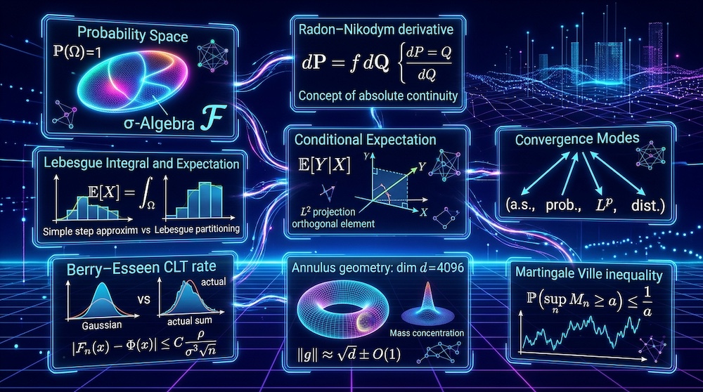
Start with the one sentence everything else hangs on, stated with the two words that are usually dropped. A probability is a measure — a countably additive function from a σ-algebra of events to $[0,1]$ with $P(\Omega) = 1$ — and a random variable is a measurable function on that space. Nothing else is primitive. "Random", "uniform", "given", "independent", "converges" and "expected" are all defined in terms of those two objects, and every time one of them produces a paradox it is because the measure or the σ-algebra was left implicit and two readers filled it in differently. Draw a "random chord" of a circle and ask how often it is longer than the inscribed triangle's side: three natural constructions give $\tfrac13$, $\tfrac12$ and $\tfrac14$, and all three are correct, because "random chord" named no measure. Condition a uniformly random point on a sphere on its lying on a great circle, and the answer depends on which family of events shrinks to that circle — a band of latitude gives a uniform law on the circle, a band of longitude gives one proportional to the cosine of latitude. §0 shows both with numbers. Every result in this piece is a consequence of taking that sentence seriously, including the cases where a quantity that looks like a probability is a density and can exceed one, and where a sequence that "converges" does so in a mode that licenses nothing you wanted.

Here is the claim, at the width the mathematics supports, because the tidy version is wrong in both directions. We are not claiming that machine learning is measure theory wearing a hat, and we are not claiming that a practitioner needs to see a non-measurable set to train a model — nobody meets one, and we say exactly where the σ-algebra stops mattering. The claim is this:

Probability theory supplies the objects that every training claim is a statement about, and the mode in which each claim is true. "The MSE-optimal predictor is the conditional mean" is an exact theorem about an $L^2$ projection. "SGD converges" is true almost surely under Robbins–Monro conditions and false in that mode at a constant step under persistent gradient noise. "The sample mean is within one standard error" is a central-limit statement that the law of the iterated logarithm says fails infinitely often. "A long rollout estimates the stationary distribution" is an ergodic theorem with a precondition the episodic case violates. "Random vectors in $d = 4096$ are nearly orthogonal" is a concentration inequality with a number attached. The value of the lens is not that everything is secretly probability. It is that it tells you which of your claims are theorems, which are theorems in a weaker mode than you assumed, and which are hypotheses.

Companion notebooks. Every number in this piece is a printed line of worked_numbers.py (53 numbered sections, NumPy only, seeded), and the sections reproduce cell by cell in three executed notebooks: 00_probability_from_scratch.ipynb (§1–§14, with the companion basics' A1–A18), 01_concentration_and_chains.ipynb (§15–§53) and 02_fast_path.ipynb (the fourteen fast-path stops only).

Every connection in this piece carries one of four labels — the same four as our Information Domain piece, so the two can be read as chapters of one book. If you are here for the eval error bar, skip to §7 and come back to this table the first time a label stops you:

Where a connection has two parts we grade both: the theorem, and the claim that the machine-learning object satisfies its hypotheses. Gaussian concentration is L1; "trained embeddings satisfy it" is L3; the two grades sit side by side in §7, §6 and §9 rather than being averaged into one.

Four running examples carry the same numbers through the whole piece, so that when two sections seem to disagree you can see which one is wrong.

• E1 — the fair coin and its sequence space $\{0,1\}^{\mathbb N}$: the object that needs an extension theorem to exist (§1), the first home of the strong law and the law of the iterated logarithm (§5), the typewriter sequence (§5), the test martingale a peeking analyst cannot beat (§8).
• E2 — a two-class Gaussian mixture in $d = 20$ dimensions, class means $\pm\mu\,e_1$ with $\mu = 1$, identity covariance, equal priors: its Bayes classifier and Bayes risk $\Phi(-\mu) = 0.1587$ in closed form (§4), logistic regression's learning curve against that floor (§4), the eval-set error bar on it (§7), and SGD's iterates on it under four step-size schedules (§8).
• E3 — the standard Gaussian vector in $d$ dimensions: the norm that concentrates at $\sqrt d$ with a standard deviation that does not grow (§7), cosines that shrink as $1/\sqrt d$ (§7), the Johnson–Lindenstrauss projection (§7), covariance estimation at five sample sizes (§7), and the infinite-width network whose output is a Gaussian by the central limit theorem (§6).
• E4 — the AR(1) process at $\phi = 0.9$ and its continuous-time twin, the Ornstein–Uhlenbeck diffusion: the stationary chain whose time average has a computable variance inflation of $19\times$ (§9), the Langevin sampler whose Euler discretisation is biased by a closed-form factor (§9), the forward process of a diffusion model and its exact time reversal (§9), and the same AR(1) our Information Domain piece used for its entropy rate.

Prerequisites. Calculus, including limits of sequences; linear algebra at the level of eigenvalues; the words "mean" and "variance"; gradient descent. No measure theory is assumed, and some is taught: §1 to §3 build the four objects the rest of the piece is written in — the σ-algebra, the measurable function, the Lebesgue integral and the Radon–Nikodym derivative — from those prerequisites, and build only those; a reader meeting them for the first time should expect §1 to §3 to be the slowest sections, not the easiest, and the fast path below is for the reader who would rather take the objects on trust and return for them. Two kinds of section follow. §1 to §5, §7 and §8 are built from the stated prerequisites: each theorem they use is stated with its hypotheses and either proved, sketched, or reduced to a named result the text has already given. §6.5–§6.6, §9.3–§9.4, §10.2–§10.3 and §11 state theorems with their assumptions and a reference and do not pretend to prove them; those sections are read for what a theorem licenses and what it does not, and they are marked optional in the paths below. If you know measure theory, §1 to §3 are a fast re-read with the machine-learning consumers attached; the new material for you starts at §4.

Three reading paths, and the sections none of them may skip. The piece is six modules — Foundations §1–§4; Limits §5–§7.1; Evaluation §7.6, §8.2 and Appendix C.1; Optimisation §3.3 and §8.4; Sampling §9; Advanced §6.5–§6.6, §9.4, §10 and §11, the last of these optional — and the paths are routes through them.

The fast path, for the practitioner who wants the eval error bar and the SGD claim and will come back for the objects, has fourteen stops, each marked by a banner under its heading: §0, §2.2, §2.3, §2.4, §3.3, §4.2, §5.1, §5.4, §7.6, §8.2, §8.3, §8.4, §12 and §13, in that order. Its destination is §7.6, the eval error bar, which is stop 9; the numbers quoted at the fourteen stops run on their own in 02_fast_path.ipynb. If you only have two hours, start here and stop at §13. The fast path is a route through fourteen selected results, not a substitute for the objects behind their proofs: a claim quoted at a stop is proved in a section the path skips, and the hypotheses the stop's number rests on are stated there.

The full practitioner path is §0 → §1 → §2 → §3 → §4 → §5 → §7 → §8 → §12 → §13, doing the checkpoint exercises that lie on it. The theorist path is §0 → §1 → §2 → §3 → §4 → §5 → §6 → §7 → §8 → §9 → §10 → §11. §1 through §5 are on both full paths: §1 and §2 are the objects, §3 is why your gradient estimator is allowed to exist, §4 is the one theorem a practitioner uses every day without naming it, and §5 is the vocabulary in which every later claim is stated. §6 (the central limit theorem as a Fourier theorem) is the bridge to our frequency-domain pieces and is where a practitioner who liked those should go. §9 (chains, ergodicity, Langevin, diffusion) and §10 (minimax and the price of a density) are the advanced branches, optional on every path; take them by interest. §11 (conditional independence and exchangeability), also optional, is the on-ramp to a forthcoming piece on Bayesian and non-parametric inference and can be read on its own. The history is Appendix A, the audit of where this machinery is load-bearing outside machine learning is Appendix B, two toy cases of ours are Appendix C, and the graded ledger of how this piece bears on our earlier posts is Appendix D. This piece stands alone: where an earlier post of ours is relevant it is linked as a citation, the way a paper would be, and nothing below requires having read it.

Companion code. Every number in a code block below is copied from the printed output of worked_numbers.py, a single NumPy script with 53 numbered sections, float64, CPU-only, that ships with this piece; a section number in the form §N beside a block names the section that printed it, the numbers are verbatim, and where a line's label has been shortened for the page the full label is in the script's output file. The script's shared generator is seeded once, default_rng(20261022), and §1 to §31 draw from it in order; §32 to §53, added across four rounds of external review, each draw from a generator of their own (seeded 2026_1016_NN for section NN) and never from the shared one, so that adding them left the §1–§31 output byte-identical. Every Monte Carlo value in §1 to §53 that is compared to a theory value is printed with its standard error, computed from the draws the section already makes; the one block whose quantity has no finite variance (§11, the Pareto block means) says so in place of a bar. A test_worked_numbers.py beside the script re-derives the closed-form values the blocks are compared against. The two companion notebooks — 00_probability_from_scratch.ipynb (measure, random variable, conditioning, the four convergences, the CLT by characteristic functions, concentration) and 01_concentration_and_chains.ipynb (eval error bars, the peeking experiment, the AR(1) and Metropolis chains, Langevin, the diffusion reversal, the infinite-width network) — ship beside it, built from those sections cell by cell; each cell restores the script's generator state at its section, so a notebook prints this piece's numbers whether it is run top to bottom or one cell at a time. A third, 02_fast_path.ipynb, runs only the sections quoted at the fourteen fast-path stops, in the order of the path, with the same state restore.

Units and conventions, once. Logarithms are natural and divergences are in nats unless a line says bits — this is a probability piece, and every theorem below is stated with $\ln$; our Information Domain piece worked in bits and said so at every table. "a.s." means almost surely: with probability one. $\Phi$ is the standard normal distribution function. $\mathbb 1_A$ is the indicator of the event $A$. $\sigma(X)$ is the σ-algebra generated by $X$, defined in §1. We write $X_n \to X$ with the mode attached whenever it matters, which is every time in §5 and §8.

0. Three puzzles that are one puzzle

Fast path · stop 1 of 14. Next stop: §2.2. This section's numbers run in 02_fast_path.ipynb.

Probability is counter-intuitive in a specific way. The puzzles that trip people up are almost never about computation; they are about which question is being asked. Three of them, each resolved by naming the object the question left out, and each the seed of a section below.

Bertrand's chord (1889). Draw a chord of the unit circle "at random". The inscribed equilateral triangle has side $\sqrt 3$; how often is the chord longer? Three constructions, each uniform in some variable, each a legitimate probability measure on the set of chords:

§1  1,000,000 chords per construction
    (a) two uniform endpoints        P(L > sqrt3) = 0.3324   (theory 1/3)
    (b) uniform distance to centre   P(L > sqrt3) = 0.4994   (theory 1/2)
    (c) uniform midpoint in the disc P(L > sqrt3) = 0.2491   (theory 1/4)
    (SE of the three lines above: ± 0.0005, ± 0.0005, ± 0.0004 — binomial sqrt(p(1-p)/N) at N = 1,000,000; the largest |measured - theory| is 2.0 SE)

None of these is wrong. "Uniform" is not a property of a set; it is a property of a measure on a set, and the set of chords carries three natural ones that disagree. The lesson is not "probability is ambiguous". It is that a probability question is a question about a specified measure, and when a machine-learning claim says "sample uniformly from the data manifold", "a random initialisation", or "an uninformative prior", it has either specified the measure or it has not yet said anything. §1 makes the object precise; §10 returns to the uninformative prior.

Monty Hall (1975). Three doors, one car. You pick door 1; the host, who knows where the car is and always opens a goat door you did not pick, opens door 3. Switch?

§2  1,000,000 games: stay wins = 0.3332   switch wins = 0.6668   (theory 1/3, 2/3)
    (SE of the line above: ± 0.0005 for either frequency — binomial sqrt(p(1-p)/N) at N = 1,000,000)

The number is not the puzzle. The puzzle is that "the host opened door 3" is being conditioned on, and the probability of that event depends on the host's rule — on what he would have done had the car been behind door 1 (open 2 or 3 at random) versus door 2 (he must open 3). A host who opens a door at random and happened to reveal a goat gives a different answer ($\tfrac12$). The event "door 3 opened" is the same event for both hosts; what differs is the measure on a sample space large enough to contain the host's choice — $P(\text{opens } 3 \mid \text{car at } 2)$ is $1$ for the knowing host and $\tfrac12$ for the ignorant one — and the measure is what encodes the mechanism. Conditioning is a computation inside a specified probability space, not on the event alone. §4 is this sentence made exact, and it is the sentence under every "condition the model on the observation" claim.

The great circle (Borel, 1909; Kolmogorov, 1933). A point is uniform on the unit sphere. Condition on its lying on a particular great circle. What is its distribution along the circle? The event has probability zero, so the elementary formula $P(A \mid B) = P(A \cap B)/P(B)$ is $0/0$, and the only way to give an answer is to pick a family of positive-probability events shrinking to the circle and take a limit. Pick the circle to be the equator and shrink a band of latitude onto it; or pick the same circle as a meridian and shrink a band of longitude onto it (the code's band $|\mathrm{lon}| < \varepsilon$ takes the half of the meridian at longitude $0$; the other half gives the same histogram by symmetry):

§6  4,000,000 uniform points on the sphere
    (i) equator via latitude band:  longitude histogram (6 bins) = [0.1659 0.1707 0.1645 0.1664 0.1645 0.168 ]
    (ii) meridian via longitude band: latitude histogram (6 bins)  = [0.0665 0.1833 0.2528 0.2468 0.1876 0.0631]
         cos(latitude) at bin centres, normalised                  = [0.067  0.183  0.25   0.25   0.183  0.067 ]

Same curve on the sphere, two conditional densities: uniform in the first limit, proportional to $\cos(\text{latitude})$ in the second. Neither is "the" conditional distribution given the circle, because there is no such thing; there is a conditional distribution given a σ-algebra, and the two bands generate different ones. §4 states the theorem that resolves this (regular conditional distributions exist, and are defined relative to a σ-algebra, not an event), and the consequence for anyone who conditions a model on an exact continuous observation — an inpainting mask, a constraint — is to write down the observation model. A regular conditional distribution exists in every case (§4.4); what the paradox turns on is whether its value at one specific $x$ is pinned down, and that is a property of the conditional kernel's regularity in $x$, not of whether the joint law has a density. A singular joint law can have a perfectly regular kernel: $(X, Y) = (Z, Z)$ is singular with respect to area in the plane, yet $P(Y \in \cdot \mid X = x) = \delta_x$ at every $x$, weakly continuous in $x$, and every shrinking interval of $X$ around $x$ agrees on it. A law with a continuous joint density has the canonical version $p(y \mid x) = p(x, y)/p_X(x)$ wherever $p_X(x) > 0$, under the domination condition §4.4 states; singularity alone decides nothing in either direction. So the consequence for a generative model with a low-dimensional latent (§2.2) is not "its law is singular, so no canonical version exists" but "whether its kernel at the observed coordinates has a continuous version is a property of that learned pushforward, and one you have not verified" — which is why the observation model has to be stated; §4.4 separates that from the algorithmic differences between guidance methods, which are not of this kind.

The three puzzles are one puzzle. In each, a word that sounds primitive — random, given, on — hides a choice of measure or of σ-algebra, and the arithmetic cannot be done until the choice is made. The rest of this piece is the machinery for making those choices explicit, and then the theorems that become available once they are.

1. A probability is a measure, and the σ-algebra is the list of questions

Not on the fast path. The practical destinations — the eval error bar (§7.6) and the SGD claim (§8.4) — do not depend on this section; it supplies the objects those claims are stated in — the σ-algebra, the filtration and the almost-sure mode — for the reader who wants to see what they rest on.

1.1 The three axioms, and why "countably" is the whole point

Kolmogorov's 1933 definition. A probability space is a triple $(\Omega, \mathcal F, P)$:

• $\Omega$ is a set, the sample space — the set of everything that could happen, at whatever resolution you choose to describe it;
• $\mathcal F$ is a σ-algebra on $\Omega$: a collection of subsets, called events, that contains $\Omega$, is closed under complement, and is closed under countable unions (hence countable intersections);
• $P: \mathcal F \to [0,1]$ is a probability measure: $P(\Omega) = 1$, and for any sequence of pairwise disjoint events $A_1, A_2, \dots$ in $\mathcal F$, $$P\Big(\bigcup_{n} A_n\Big) = \sum_n P(A_n).$$

That last property, countable additivity, is the one that does the work, and it is the one that elementary treatments quietly replace with finite additivity. The difference is not pedantry. Countable additivity is equivalent, given finite additivity, to continuity: if $A_n \uparrow A$ then $P(A_n) \uparrow P(A)$, and if $A_n \downarrow A$ then $P(A_n) \downarrow P(A)$.

Continuity is what lets a probability pass through a limit — and every limit theorem in this piece, from the strong law to the martingale convergence theorem, is a statement that some sequence of events has a probability that converges to the probability of a limiting event. Drop countable additivity and the strong law of large numbers is not false; it is unstatable, because "the running mean converges" is a countable intersection of countable unions of events, which lies outside the algebra of finite-dimensional cylinder sets, and finite additivity alone determines no value for it.

A measure that is not required to total one is just a measure; Lebesgue measure $\lambda$ on $\mathbb R$, which assigns to an interval its length, is the one that will matter. Everything in this subsection holds for σ-finite measures, with one exception: continuity from above needs some $A_n$ of finite measure ($[n, \infty) \downarrow \emptyset$ while $\lambda([n, \infty)) = \infty$ for every $n$). That is why the same machinery serves densities (§2) and integrals (§3).

1.2 Why not every subset: the one pathology, and then never again

Why does the definition need $\mathcal F$ at all? Why not let every subset of $\Omega$ be an event? For a finite or countable $\Omega$ you can, and should: $\mathcal F = 2^\Omega$, and a probability is a list of non-negative numbers summing to one. The need arises on $[0,1]$, and it arises from a theorem.

Vitali (1905). There is no function $\mu: 2^{[0,1]} \to [0,\infty]$ that is countably additive, translation-invariant (modulo 1), and assigns $[0,1]$ the value one.

Optional — why the σ-algebra is forced. The sketch, for the reader who wants to see the set. Call $x \sim y$ if $x - y$ is rational, and use the axiom of choice to pick one representative from each equivalence class; call the set of representatives $V$. The rational translates $V + q$ (mod 1), $q \in \mathbb Q \cap [0,1)$, are countably many, pairwise disjoint, and cover $[0,1)$ — which has the same measure as $[0,1]$, since a single point has countably many disjoint translates of equal measure inside $[0,1]$ and so has measure zero. By countable additivity and translation invariance, $1 = \mu([0,1)) = \sum_q \mu(V+q) = \sum_q \mu(V)$ — a countable sum of a single number, which is $0$ or $\infty$, never $1$.

So a "uniform distribution on $[0,1]$" in the only sense that supports limits cannot be defined on every subset. It can be defined on the Borel σ-algebra $\mathcal B$ — the smallest σ-algebra containing the intervals — and, slightly larger, on the Lebesgue-measurable sets.

Every set you will ever write down (intervals, their countable unions and intersections, preimages under continuous or Borel-measurable functions, limits of all of these) is Borel — under a merely Lebesgue-measurable function the preimage of a Borel set is Lebesgue-measurable, not necessarily Borel, which is all this section needs — and the one exception is forward images and projections (Suslin, 1917: the projection of a Borel subset of the plane is analytic, hence Lebesgue-measurable, but not always Borel).

The Vitali set needs the axiom of choice to exist and cannot be described by a rule. A practitioner will never meet a non-measurable set, and this is the last time this piece mentions one. The σ-algebra is forced by Vitali, but once it is there it does a second job that has nothing to do with pathology, and that second job is why it stays in the definition.

1.3 The second job: a σ-algebra is information

Take a random variable $X$ (defined in §2; for now, a function $\Omega \to \mathbb R$ whose preimages of intervals are events). The σ-algebra generated by $X$,

is the collection of events that can be decided by looking at $X$ alone — "$X > 3$", "$X \in [0,1] \cup [2,5]$", "$X$ is rational" — and not the events that cannot, like "$Y > 3$" for an unrelated $Y$. A sub-σ-algebra $\mathcal G \subseteq \mathcal F$ is in general a list of questions you are allowed to ask, closed under and, or, not, and countable versions of these. Three consequences, each a section of this piece:

1. A function of the data is the same thing as a $\sigma(\text{data})$-measurable function. This is the Doob–Dynkin lemma: a random variable $Z$ is $\sigma(X)$-measurable if and only if $Z = g(X)$ for some Borel function $g$. It is what makes "a predictor that depends only on the input" a mathematical object, and it is what §4 projects onto.
2. Information over time is an increasing sequence of σ-algebras, a filtration $\mathcal F_1 \subseteq \mathcal F_2 \subseteq \cdots$, where $\mathcal F_n$ is what is decidable after $n$ steps. "A stopping rule that does not look into the future" means a random time $\tau$ with $\{\tau \le n\} \in \mathcal F_n$ for every $n$. That single line is the definition under every early-stopping, checkpoint-selection and sequential-testing argument in §8.
3. Independence is a statement about σ-algebras: $X$ and $Y$ are independent when $P(A \cap B) = P(A)P(B)$ for every $A \in \sigma(X)$ and $B \in \sigma(Y)$, and conditional independence (§11) is the same with a third σ-algebra conditioned on. "Independent" is not a property of two numbers; it is a property of two lists of questions.

1.4 Existence: three theorems that let you say "an i.i.d. stream" at all

Here is a question that sounds silly and is not. E1 is an infinite sequence of fair coin flips. Does a probability space carrying it exist? Finite additivity on finite sequences is easy — $2^{-n}$ to each of the $2^n$ strings. The infinite sequence space $\{0,1\}^{\mathbb N}$ is uncountable, every individual infinite string must have probability zero, and the measure has to be countably additive on a σ-algebra large enough to contain "the running mean converges to $\tfrac12$", which is not a statement about any finite prefix. Three theorems, in increasing generality:

Carathéodory's extension theorem. A non-negative countably additive set function on an algebra (closed under finite operations) — a premeasure — extends to a measure on the σ-algebra it generates, uniquely when it is σ-finite. Together with the π–λ theorem (Dynkin): two probability measures that agree on a collection closed under finite intersections — a π-system — agree on the σ-algebra it generates. The second half is the one practitioners use without knowing: specifying a distribution function $F(x) = P(X \le x)$ specifies the whole law, because the half-lines $(-\infty, x]$ form a π-system generating $\mathcal B$. Likewise specifying $P(X_1 \le x_1, \dots, X_n \le x_n)$ specifies a joint law.

Product measure. Given probability spaces for $X$ and for $Y$, there is exactly one measure on the product σ-algebra under which $P(A \times B) = P(A)P(B)$. "A dataset of $n$ independent samples" is a point of the $n$-fold product space, and "i.i.d." is the statement that the joint law is the product of $n$ copies of one marginal. Fubini's theorem (§3) is the theorem about integrating against a product measure.

Kolmogorov's extension theorem (1933). Three things you want to be allowed to say, and this is the theorem that allows them: that a product measure exists for infinitely many factors, so an i.i.d. stream is an object and not only an $n$-sample; that any consistent family of marginals is the family of some process, so "a stochastic process with these finite-dimensional laws" names something; and that all of these live on one space $\Omega$, which an almost-sure statement about the whole sequence — E1's running mean converging — needs in order to be an event at all.

The statement: given a consistent family of finite-dimensional distributions — a law for $(X_1, \dots, X_n)$ for every $n$, each the marginal of the next — there is a unique probability measure on $\mathbb R^{\mathbb N}$ (with the σ-algebra generated by the coordinates) having those marginals. This is the theorem that makes E1 exist, and with it every "infinite stream of training batches", every "stochastic process", every Markov chain of §9. (On general spaces it needs the coordinate spaces to be standard Borel — Polish spaces with their Borel sets — which every space in this piece is.)

At a glance — the three theorems, what each takes in and what it hands back:

The point of listing these is not that you will invoke them. It is that the i.i.d. assumption is a construction, not an observation: the product measure is an object you chose, and the theorems below are theorems about that object. When the data are not a product — a time series, a conversation, a sequence of agent actions — the object is a different measure on the same sequence space, and §9 and §11 are about which theorems survive.

1.5 Almost surely, and the two Borel–Cantelli lemmas

An event $A$ holds almost surely (a.s.) if $P(A) = 1$. It is not "surely": the complement is non-empty, merely null. A uniform variable on $[0,1]$ takes some value, and takes any particular value with probability zero. The rationals are dense in $[0,1]$ — every interval contains infinitely many — and have Lebesgue measure zero, being a countable union of points:

§3  Riemann upper sum = 1, lower sum = 0 on every partition -> not Riemann integrable
    Lebesgue: lambda(Q cap [0,1]) = 0  ->  integral of 1_Q = 0  (a countable union of points)

So "a uniform draw is irrational" holds a.s. and is not certain, and the indicator of the rationals — a function that is $1$ on a dense set — integrates to zero. That last line is also the first hint of why the integral of §3 is Lebesgue's and not Riemann's: the Riemann integral of $\mathbb 1_{\mathbb Q}$ does not exist, and the Lebesgue integral is $0$ without fuss.

Two lemmas about infinitely many events, used constantly below. Write $\{A_n \text{ i.o.}\}$ — infinitely often — for $\limsup_n A_n = \bigcap_m \bigcup_{n \ge m} A_n$, the event that infinitely many $A_n$ occur.

• Borel–Cantelli I. If $\sum_n P(A_n) < \infty$ then $P(A_n \text{ i.o.}) = 0$. No independence needed. This is how almost-sure convergence is usually proved: show the probabilities of the bad events are summable.
• Borel–Cantelli II. If the $A_n$ are independent and $\sum_n P(A_n) = \infty$ then $P(A_n \text{ i.o.}) = 1$.

Together: for independent events, "infinitely often" has probability $0$ or $1$, decided by a single series. That is a special case of Kolmogorov's 0–1 law: any event in the tail σ-algebra of an independent sequence — any event unchanged by altering finitely many of the $X_n$ — has probability $0$ or $1$. "The running mean $S_n/n$ converges" is a tail event, so for an i.i.d. sequence the strong law of §5 is either true a.s. or false a.s.; there is no middle. Whether the iterates of a stochastic optimiser converge is not in general a tail event — the early steps matter — which is one reason §8 needs martingales rather than a 0–1 law.

Checkpoint exercise 1a. E1 again. (i) Fix a finite pattern — say ten heads in a row. Does it occur infinitely often along the sequence, almost surely, and which Borel–Cantelli lemma decides it? (ii) Write $\mathcal F_n = \sigma(X_1, \dots, X_n)$, heads $= 1$. Is the event $\{\text{first head at time } 3\}$ in $\mathcal F_2$? In $\mathcal F_3$? (Answers: (i) Yes, a.s. Overlapping occurrences are not independent, so cut the sequence into disjoint blocks of ten and let $A_k$ be "block $k$ is all heads": the $A_k$ are independent with $P(A_k) = 2^{-10}$, the series diverges, and Borel–Cantelli II gives $P(A_k \text{ i.o.}) = 1$; infinitely many full blocks are infinitely many occurrences. Borel–Cantelli I says nothing here: its hypothesis, a summable series, fails. (ii) No: $\{\text{first head at time } 3\} = \{X_1 = 0, X_2 = 0, X_3 = 1\}$ is decided by $X_3$, which $\mathcal F_2$ cannot ask about; it is in $\mathcal F_3$ — compare §1.3's stopping-time definition.)

1.6 Where this touches a loss function already

Our Information Domain piece opened with the typical set: for an i.i.d. source, the sequences whose empirical log-probability is close to the entropy have total probability tending to one while being an exponentially vanishing fraction of all sequences — for a source that is not uniform; a uniform source has $H = \ln|\mathcal X|$, every sequence is typical, and the two agree.

In this section's vocabulary that is a statement about a measure on E1's sequence space — a set of sequences that is small as a set and large in measure — and the asymptotic equipartition property it rests on is the strong law of large numbers applied to $-\log p(X_i)$, which §5 states and §9 extends from i.i.d. to ergodic. The point for now is only that "most sequences" in machine learning always means "most of the measure", never "most of the set", and the two can disagree by a factor of $e^{n(\ln|\mathcal X| - H)}$.

The objects you actually need, on one page. Ten of them carry the whole piece; the table says what each is in one line and where it is defined, so that a later section can be read without re-deriving its vocabulary.

Every later section refers back to this table; if a term is opaque, return here.

Checkpoint exercise 1b. Let $X$ be a fair coin flip and $Y$ an independent fair die. Which of these events are in $\sigma(X)$: (a) $\{X = 1\}$; (b) $\{X = 1, Y = 3\}$; (c) $\{Y \text{ is even}\}$; (d) $\Omega$; (e) $\{X = 1\} \cup \{Y = 6\}$? Then: is "$S_n/n \to \tfrac12$" a tail event for E1, and is "$S_n > 0$ for all $n$"? (Answers: (a), (d); yes — altering finitely many flips does not change the limit; no — altering the first flip can break it.)

2. A random variable is a function; a density is a derivative

2.1 Measurable maps and pushforward: where "the distribution of $X$" lives

A random variable (§1.6 glossary) is a function $X: \Omega \to \mathbb R$ that is measurable: $X^{-1}(B) \in \mathcal F$ for every Borel set $B$. Measurability is the condition that lets $P$ be applied to statements about $X$, and it is almost never a constraint in practice — every continuous function, every function built from continuous functions by countable limits, every function you can write in a framework is measurable. A random vector is the same with $\mathbb R^d$; a random element of any standard Borel space (a function space, a space of images, a set of token sequences) is the same with that space.

The law or distribution of $X$ is the pushforward measure (§1.6 glossary) $P_X = P \circ X^{-1}$ on $\mathbb R$: $P_X(B) = P(X \in B)$. The distribution function is $F_X(x) = P_X((-\infty, x])$, and by the π–λ theorem of §1.4 it determines $P_X$. The one identity that practitioners use ten times a day and textbooks call "the law of the unconscious statistician" is the change-of-variables formula for the pushforward,

valid for Borel $g$ with $g \ge 0$ or $g(X)$ integrable, which says you may forget $\Omega$ and integrate over the range. It is a theorem (prove it for indicators, then simple functions, then by the limit theorems of §3), and it is the reason a model only ever needs the law of its data and not the sample space (§1.6 glossary) the data were drawn on.

$\Omega$ is scaffolding. No computation in machine learning ever refers to $\Omega$; everything is a statement about laws, which is why the pushforward is the first thing to define. The scaffolding matters at exactly two moments: when a limit theorem needs several random variables to live on one space (§5's almost-sure convergence is a statement about $\omega$-by-$\omega$ convergence, which has no meaning without a shared $\Omega$), and when two constructions produce the same law but different joint behaviour — a coupling, two random variables on one $\Omega$ with prescribed laws, which is how §2.4's Wasserstein distance is defined.

Checkpoint exercise 2a. Let $U$ be uniform on $[-1, 1]$ and $X = U^2$. (i) Find the law of $X$ — its distribution function and its density. (ii) Is $\sigma(X) \subsetneq \sigma(U)$? Name an event in one and not the other. (Answers: (i) For $x \in [0,1]$, $P(X \le x) = P(-\sqrt x \le U \le \sqrt x) = \sqrt x$, so $F_X(x) = \sqrt x$ and the pushforward $P_X$ has density $p_X(x) = \tfrac{1}{2\sqrt x}$ on $(0, 1]$: it is $5$ at $x = 0.01$ and $50$ at $x = 10^{-4}$, unbounded as $x \downarrow 0$, and still $\int_0^1 \tfrac{dx}{2\sqrt x} = 1$ — a density is a Radon–Nikodym derivative, not a probability (§2.2). (ii) Yes, strictly. Every event in $\sigma(X)$ has the form $\{U^2 \in B\}$ and is unchanged by the reflection $U \mapsto -U$; the event $\{U > 0\}$ is in $\sigma(U)$ and is sent by that reflection to $\{U < 0\}$, a different event, so it is not in $\sigma(X)$. In the words of Doob–Dynkin (§1.3), $\mathrm{sign}(U)$ is not a Borel function of $U^2$: knowing the square cannot decide the sign, and squaring threw a question off the list.)

2.2 Densities: absolute continuity and the Radon–Nikodym derivative

Fast path · stop 2 of 14. Next stop: §2.3. This section's numbers run in 02_fast_path.ipynb.

A density is not primitive either. Given two measures $\mu$ and $\nu$ on the same space, say $\mu$ is absolutely continuous with respect to $\nu$, written $\mu \ll \nu$ (§1.6 glossary), if every $\nu$-null set is $\mu$-null: $\nu(A) = 0 \Rightarrow \mu(A) = 0$. Then:

Radon–Nikodym theorem. If $\mu \ll \nu$ and both are σ-finite, there is a $\nu$-a.e. unique measurable $f \ge 0$ with

written $f = d\mu/d\nu$. Conversely if $\mu$ is given by such an $f$ then $\mu \ll \nu$.

A probability density function (§1.6 glossary: the density as a Radon–Nikodym derivative) is the case $\nu = \lambda$, Lebesgue measure: $p_X = dP_X/d\lambda$ exists exactly when $P_X$ assigns zero to every set of length zero. A probability mass function is the case $\nu =$ counting measure on a countable set. These are the same object with respect to different base measures, and three facts that cause real errors follow immediately:

• A density is not a probability. It is a derivative — a ratio of a probability to a length — and can exceed one; $\mathcal N(0, \sigma^2 = 0.01)$ has density $\approx 3.99$ at zero. A model's log-likelihood on continuous data is not bounded above by zero.
• A density depends on the base measure, so likelihoods are comparable only against the same one. The log-likelihood of a continuous model on data that are actually discrete (8-bit pixels, quantised audio) is not a well-posed number: the data law is a sum of point masses, which is singular with respect to Lebesgue measure, and a continuous model can drive its density at the data points to infinity by concentrating mass there. Theis, van den Oord & Bethge (2016) make this point and the field's fix — dequantisation, adding uniform noise in the quantisation cell so that the data law becomes absolutely continuous — is exactly "choose a data measure that is $\ll \lambda$ before you compare densities". Reporting bits per dimension is then a well-defined comparison between models under the same dequantised measure, and only that. L1.
• A law can have no density at all and still be perfectly good. The Lebesgue decomposition says that for σ-finite $\mu$ and $\nu$, $\mu$ splits uniquely as $\mu_{\mathrm{ac}} + \mu_{\mathrm{sing}}$ with $\mu_{\mathrm{ac}} \ll \nu$ and $\mu_{\mathrm{sing}} \perp \nu$ (concentrated on a $\nu$-null set); the singular part further splits into atoms (point masses) and a singular-continuous part. A spike-and-slab prior, a zero-inflated count model, an image distribution with saturated pixels, and the law of any generative model that maps a low-dimensional latent through a smooth decoder into a high-dimensional space all have singular parts — the last one is singular with respect to Lebesgue measure on $\mathbb R^D$ entirely, since its mass lives on a $d$-dimensional image, a $\lambda_D$-null set. That observation is the whole of §2.4.

2.3 Change of variables, and what a normalising flow computes

Fast path · stop 3 of 14. Next stop: §2.4. This section has no numeric block; the stops' numbers run in 02_fast_path.ipynb.

If $X$ has density $p_X$ on $\mathbb R^d$ and $T: \mathbb R^d \to \mathbb R^d$ is a diffeomorphism, then $Y = T(X)$ has density

This is the Radon–Nikodym derivative of the pushforward $P_X \circ T^{-1}$ with respect to Lebesgue measure, and the Jacobian is the factor by which $T$ rescales volume — Lebesgue measure is not preserved by a general map, and the density has to account for that.

A normalising flow is a parametrised diffeomorphism trained by maximising this expression at the data; the architecture constraints (triangular Jacobians, coupling layers) exist to make $\det J$ cheap.

If $T$ is not injective but is still a local diffeomorphism off a null set, the formula becomes a sum over the preimage branches; it fails entirely when $T$ sends a set of positive $P_X$-measure into a $\lambda$-null set — as any map into a space of higher dimension must — which is the formal reason a decoder from $\mathbb R^d$ to $\mathbb R^D$ with $d < D$ produces a law without a density on $\mathbb R^D$, and why a VAE needs the noise in $p(x \mid z)$ to have a density at all. (Our Information Domain piece's §6 took that density as given; this is where it comes from.)

Checkpoint exercise 2b. $X \sim \mathcal N(0,1)$ with density $\varphi$, and $Y = e^X$. (i) Write the density of $Y$ by the change-of-variables formula. (ii) Can it exceed one? If not, find a $Y' = e^{X/c}$ whose density does, and say what the extra factor is. (Answers: (i) $T(x) = e^x$ is a diffeomorphism of $\mathbb R$ onto $(0, \infty)$ with $T^{-1}(y) = \ln y$ and $|dT^{-1}/dy| = 1/y$, so $p_Y(y) = \varphi(\ln y)/y$ for $y > 0$ — the lognormal density; the $1/y$ is the Jacobian, the factor by which $T$ stretches length near $y$. (ii) Not this one: $\ln p_Y$ is maximised where $-\ln y - \tfrac12(\ln y)^2$ is, at $\ln y = -1$, and $p_Y(e^{-1}) = \varphi(-1)\,e = 0.242 \times 2.718 = 0.658$. Compress instead: $Y' = e^{X/4}$ has $T^{-1}(y) = 4\ln y$ and $p_{Y'}(y) = 4\,\varphi(4\ln y)/y$, so $p_{Y'}(1) = 4\varphi(0) = 1.596$, the peak is $1.646$ at $y = e^{-1/16} = 0.939$, and $p_{Y'} > 1$ on roughly $[0.732, 1.206]$ — while $\int_0^\infty p_{Y'}\,dy = 1$ exactly, since the formula is the Radon–Nikodym derivative of the pushforward with respect to Lebesgue measure and the pushforward is a probability. A density above one is a short interval carrying a lot of mass, not an error, and the $4/y$ that put it there is exactly the $\log|\det J|$ term a normalising flow adds to its log-likelihood.)

2.4 Divergences as integrated density ratios, and the support problem

Fast path · stop 4 of 14. Next stop: §3.3. This section's numbers run in 02_fast_path.ipynb.

With the Radon–Nikodym derivative in hand, the divergences of our earlier piece are one-line definitions. For probability measures $P, Q$:

The "otherwise" is not a convention; it is forced. If $P$ puts mass on a $Q$-null set, no density $dP/dQ$ exists and the integral has an infinite part. Three other divergences, each needing less:

• Total variation $\mathrm{TV}(P, Q) = \sup_A |P(A) - Q(A)|$: always defined, always in $[0,1]$, equal to $\tfrac12 \int |p - q|\,d\nu$ for any common dominating $\nu$ (which always exists: $\nu = P + Q$).
• Jensen–Shannon $\mathrm{JS}(P,Q) = \tfrac12 \mathrm{KL}(P \| M) + \tfrac12 \mathrm{KL}(Q \| M)$ with $M = \tfrac12(P+Q)$: always finite, since $dP/dM = 2p/(p+q) \le 2$ and likewise $dQ/dM \le 2$ — the log-ratios are bounded above by $\ln 2$, not merely defined — and capped at $\ln 2$.
• Wasserstein-1 $W_1(P, Q) = \inf_{\gamma} \mathbb E_{(X,Y)\sim\gamma}|X - Y|$ over couplings $\gamma$ with marginals $P$ and $Q$: it needs no density ratio at all, only a metric on the space, and it is finite whenever both laws have a first moment — a sufficient condition, not a necessary one: two standard Cauchy laws shifted by $1$ have $W_1 = 1$ exactly, by the shift coupling $Y = X + 1$, while neither has a mean (§52) — and it is the one divergence here that uses the scaffolding — a coupling is a joint law with the prescribed marginals, realised as two random variables on one $\Omega$.

The textbook example, which is also the generative-modelling example (KL and JS in nats):

§20 U[0,1] vs U[theta, 1+theta]
    theta=0.0 : KL = 0.0,  TV = 0.00,  W1 = 0.00
    theta=0.01: KL = inf,  TV = 0.01,  W1 = 0.01
    theta=0.1 : KL = inf,  TV = 0.10,  W1 = 0.10
    theta=0.5 : KL = inf,  TV = 0.50,  W1 = 0.50
    theta=1.0 : KL = inf,  TV = 1.00,  W1 = 1.00,  JS = ln2 = 0.6931 (saturated)
    theta=2.0 : KL = inf,  TV = 1.00,  W1 = 2.00,  JS = ln2 = 0.6931 (saturated)

Shift a uniform law by any $\theta > 0$ and the KL is infinite immediately — the supports differ on a set of positive $P$-measure — while TV and $W_1$ grow continuously, and only $W_1$ keeps growing once the supports are disjoint.

($W_1$ is not, in general, the one that stays finite when KL does not: a first moment of each law is sufficient for finiteness, not necessary — the two shifted Cauchy laws of §52 have $W_1 = 1$ with no mean on either side — but without one it can be infinite. The Cauchy-against-Gaussian pair below has $\mathrm{KL} = \infty$ and $W_1 = \infty$ — under any coupling $\mathbb E|X - Y| \ge \mathbb E|X| - \mathbb E|Y| = \infty$ when the first law has no mean and the second does — while TV is finite; the right contrast is "no density ratio needed, finite under a first moment".)

Now take the step from the interval to the image space one object at a time. A generator $G$ with a latent $Z \sim \mathcal N(0, I_{128})$ produces samples whose law is the pushforward $P_G = \mathcal N(0, I_{128}) \circ G^{-1}$ of §2.1 — a probability measure on $\mathbb R^D$, $D = 3 \times 256 \times 256$, carried entirely by the image $G(\mathbb R^{128})$, a set of dimension at most $128$ and so of Lebesgue measure zero in $\mathbb R^D$: by the §2.3 argument $P_G$ is singular with respect to $\lambda_D$ (§2.2) and has no density there, whatever the architecture.

The law of real images is, on the manifold hypothesis, a measure of the same kind carried by a different thin set.

Two steps are being taken here, and only the first is free. That each law is singular with respect to $\lambda_D$ follows from the dimension count alone; but two laws each singular with respect to $\lambda_D$ need not be singular with respect to each other — two laws carried by the same manifold, each with a density against its surface measure, are mutually absolutely continuous and have a finite KL. Mutual singularity needs its own hypothesis on the supports, and that is the one the next paragraph makes.

Two measures carried by different Lebesgue-null sets are, generically, carried by disjoint ones — each singular with respect to the other, which is the shifted-uniform table with $\theta$ past $1$ in every direction at once — and you have Arjovsky & Bottou (2017): when the two supports are disjoint low-dimensional sets, KL is infinite, JS is at its cap $\ln 2$, a perfect discriminator exists, and the gradient the generator receives through a saturated divergence is zero or unstable.

Three claims sit in that sentence and carry different grades: that the divergence saturates is L1; that a perfect discriminator exists is L1 (the indicator of one support is one); that training therefore behaves as it does is L3 — the first two are statements about a loss surface, the third is about an optimiser on it. The divergence statement is L1 — it is a theorem about absolute continuity, with the numbers above as its one-dimensional instance.

The Wasserstein GAN of Arjovsky, Chintala & Bottou (2017) replaces the JS objective with $W_1$ via its Kantorovich–Rubinstein dual, $W_1(P,Q) = \sup_{\|f\|_{\mathrm{Lip}} \le 1} \big(\mathbb E_P f - \mathbb E_Q f\big)$ for $P, Q \in \mathcal P_1$, the laws with a finite first moment. The qualifier is load-bearing: outside $\mathcal P_1$ the coupling definition still stands — the shifted Cauchy pair has $W_1 = 1$ — but the displayed supremum is not well defined as written, because the admissible test function $f(x) = x$ has no expectation under either law; a dual over bounded Lipschitz test functions is the formulation that extends. Within $\mathcal P_1$ it is a divergence that the shifted-uniform table shows stays informative; that WGAN therefore trains better in a given setting is L3, a hypothesis about an optimiser that the theorem does not reach. Our game-theory piece treated the GAN as a minimax game; §10 says what kind of minimax it is.

Action changed — the support diagnostic. Persistent near-perfect discrimination on a sufficiently large independent evaluation sample is evidence of substantial mismatch — not proof that the supports are disjoint. A flexible discriminator memorises a finite training sample to $100\,\%$ even when $P = Q$ and the Bayes accuracy is $\tfrac12$; investigate support separation, discriminator overfitting and feature differences before diagnosing divergence saturation. If the supports are the cause, change the measures, not the model's size — add noise to both laws (instance noise, or the dequantisation of §2.2, so that both are $\ll \lambda_D$ and overlap), train against $W_1$, which stays informative once the supports are disjoint (table above), or fix the generator's support (latent dimension, decoder range). L1 that a discriminator with accuracy one on the two laws exists exactly when they are mutually singular (one direction is the indicator of a support; for the other, a classifier right with probability one under each law names a set of full $P$-measure and zero $Q$-measure); L3 that an observed near-perfect accuracy on finite samples means that, and which remedy trains best.

One inequality ties the two families together and is used in §7 and §10. Pinsker's inequality: $\mathrm{TV}(P,Q) \le \sqrt{\tfrac12 \mathrm{KL}(P\|Q)}$, KL in nats.

§20 Pinsker check on Bernoulli(0.5) vs Bernoulli(0.6): TV = 0.1, KL(nats) = 0.02041, sqrt(KL/2) = 0.1010 >= TV

It is tight to within one percent here and loose in general; its value is that it converts a KL — which is what likelihood-based training controls — into a bound on the probability of any event, which is what a downstream decision cares about.

Our Information Domain piece's §1.2 was about KL's asymmetry; this section's addition is that the asymmetry is the asymmetry of absolute continuity: $P \ll Q$ and $Q \ll P$ are different conditions, and $\mathrm{KL}(P\|Q) < \infty$ requires the first — requires, not follows from: even with a density, $\int \log\frac{dP}{dQ}\,dP$ can be $+\infty$ when $P$'s tails are heavier than $Q$'s (a Cauchy $P$ against a Gaussian $Q$ has $P \ll Q$ and infinite KL).

Checkpoint exercise 2c. $P = \mathcal N(0,1)$ and $Q$ the law of a fair coin's outcome in $\{-1, +1\}$. Which of $\mathrm{KL}(P\|Q)$, $\mathrm{KL}(Q\|P)$, $\mathrm{TV}$, $\mathrm{JS}$, $W_1$ are finite, and which are at their maximum? (Both KLs are $+\infty$: $Q$ charges $\{-1,+1\}$, which is $P$-null, so $Q \not\ll P$; $P$ charges $\mathbb R \setminus \{-1,+1\}$, which is $Q$-null, so $P \not\ll Q$. $\mathrm{TV} = 1$, $\mathrm{JS} = \ln 2$, both at their maximum. $W_1$ is finite: the optimal coupling on the line is monotone, sending $Z > 0$ to $+1$ and $Z < 0$ to $-1$, so $W_1 = \mathbb E\,\big|\,|Z| - 1\big| = 2\big[(\Phi(1) - \tfrac12) - (\varphi(0) - \varphi(1)) + \varphi(1) - (1 - \Phi(1))\big] \approx 0.54$ with $\varphi$ the standard normal density.)

3. Expectation is a Lebesgue integral, and the three theorems that let you move a gradient inside it

3.1 The construction, in three steps, and why it is not Riemann's

The expectation $\mathbb E[X] = \int_\Omega X\,dP$ is defined in three steps, and the order of the steps is the whole idea.

1. Simple functions. If $X = \sum_{k=1}^m a_k \mathbb 1_{A_k}$ for events $A_k$ and constants $a_k$, then $\mathbb E[X] = \sum_k a_k P(A_k)$. This is the only place probabilities of events enter.
2. Non-negative functions. If $X \ge 0$, then $\mathbb E[X] = \sup\{\mathbb E[S] : S \text{ simple},\ 0 \le S \le X\}$, which may be $+\infty$. Equivalently, take any increasing sequence of simple functions $S_n \uparrow X$ (one always exists: round $X$ down to multiples of $2^{-n}$ and cap at $n$) and set $\mathbb E[X] = \lim \mathbb E[S_n]$ — the monotone convergence theorem below says the limit does not depend on the sequence.
3. General functions. Split $X = X^+ - X^-$ with $X^\pm \ge 0$ and set $\mathbb E[X] = \mathbb E[X^+] - \mathbb E[X^-]$, provided at least one is finite. $X$ is integrable when $\mathbb E|X| = \mathbb E[X^+] + \mathbb E[X^-] < \infty$.

Riemann partitions the domain into intervals and asks what the function does on each; Lebesgue partitions the range into levels and asks how much measure each level set has. That is why the indicator of the rationals integrates to zero under Lebesgue and fails to exist under Riemann (§1.5): its level sets $\{\mathbb 1_{\mathbb Q} = 1\} = \mathbb Q$ and $\{\mathbb 1_{\mathbb Q} = 0\}$ have measures $0$ and $1$, and that is all the construction asks.

The practical payoff is not that integral; it is that the construction from below by monotone limits gives three theorems about exchanging a limit with an expectation, and those three theorems are what a training loop runs on.

3.2 Monotone convergence, Fatou, dominated convergence — with the counter-example that separates them

Let $X_n \to X$ almost surely — one mode of convergence (§1.6 glossary); §5.1 compares the four.

• Monotone convergence (MCT). If $0 \le X_1 \le X_2 \le \cdots$, then $\mathbb E[X_n] \uparrow \mathbb E[X]$. No integrability needed; both sides may be $+\infty$.
• Fatou's lemma. If $X_n \ge 0$, then $\mathbb E[\liminf X_n] \le \liminf \mathbb E[X_n]$. Mass can escape, never appear.
• Dominated convergence (DCT). If $|X_n| \le Y$ for all $n$ with $\mathbb E[Y] < \infty$, then $\mathbb E[X_n] \to \mathbb E[X]$ and in fact $\mathbb E|X_n - X| \to 0$.

Side by side — the hypothesis each theorem charges, what it pays, and what the escaping-mass sequence below does to it:

The example that shows the dominating function is not decoration is the escaping-mass sequence: with $U$ uniform on $[0,1]$, let $X_n = n\,\mathbb 1\{U < 1/n\}$.

§7  100,000 draws of U
    escaping mass n=   10: P(X_n != 0) = 0.0997, E[X_n] = 0.997
    escaping mass n=  100: P(X_n != 0) = 0.0104, E[X_n] = 1.039
    escaping mass n= 1000: P(X_n != 0) = 0.0011, E[X_n] = 1.110
    escaping mass n=10000: P(X_n != 0) = 0.0001, E[X_n] = 1.400
    (SE of the four lines above, from the same 100,000 points: P(X_n != 0) ± 0.0009, 0.0003, 0.0001, 0.0000;  E[X_n] = n · P(X_n != 0) here, so ± 0.009, 0.032, 0.105, 0.374 — the E[X_n] column is a mean of 100,000 terms of which only n^-1 of them are nonzero, which is why it wanders while its expectation is exactly 1)

$X_n \to 0$ for every $U > 0$, so almost surely; $\mathbb E[X_n] = 1$ for every $n$ (the Monte Carlo values wobble because by $n = 10^4$ only about ten of the $10^5$ sample points are non-zero). The limit of the expectations is $1$, the expectation of the limit is $0$, and Fatou's inequality is strict. No integrable $Y$ dominates the sequence — the smallest candidate is $\sup_n X_n$, which behaves like $1/U$ near zero and has infinite expectation.

The lesson is one sentence: a sequence of estimators can converge to the right thing almost surely while their expectations converge to the wrong thing, and the certificate that rules this out is a dominating integrable function. That certificate is what the next subsection is about.

The general principle, of which domination is the usual certificate. Call a family $\{X_n\}$ uniformly integrable if $\sup_n \mathbb E\big[|X_n|\,\mathbb 1\{|X_n| > K\}\big] \to 0$ as $K \to \infty$ — no member can keep a fixed amount of its expectation arbitrarily far out. Vitali's convergence theorem (the same Vitali as §1.2): for integrable $X_n$, $X_n \to X$ in $L^1$ with $X$ integrable if and only if $X_n \to X$ in probability and $\{X_n\}$ is uniformly integrable. That is the exact condition for the expectations to follow the limit; the DCT is its most-used sufficient case, since $|X_n| \le Y$ with $\mathbb E[Y] < \infty$ makes the family uniformly integrable at once.

The escaping-mass sequence fails it in the plainest way — $\mathbb E[X_n \mathbb 1\{X_n > K\}] = 1$ for every $n > K$, so the supremum never falls below $1$ — which is the theorem's way of saying the expectations were never going to follow the limit.

Two consequences for the rest of the piece. A family bounded in $L^p$ for some $p > 1$ is uniformly integrable (de la Vallée Poussin), which is why §5.1's table places $L^p$ convergence above convergence in probability and why a moment bound is a licence to exchange a limit with an expectation; and sub-Gaussian tails (§7) give every moment at once, so the tail and moment hypotheses of §7 and §8 are more than conveniences — they are the certificates that the quantities whose limits those sections take are uniformly integrable.

Checkpoint exercise 3a. Which of MCT, Fatou and DCT licenses $\lim_n \mathbb E[X_n] = \mathbb E[\lim_n X_n]$ for (a) the escaping-mass sequence $X_n = n\,\mathbb 1\{U < 1/n\}$; (b) the truncations $X_n = \min(X, n)$ of a random variable $X \ge 0$; (c) a sequence with $|X_n| \le c$ for a constant $c$, converging almost surely? (Answers: (a) None. The sequence is not monotone, no integrable $Y$ dominates it, and Fatou gives only $\mathbb E[\lim X_n] = 0 \le \liminf \mathbb E[X_n] = 1$ — the inequality is strict and the exchange is false. (b) MCT: $0 \le \min(X, n) \uparrow X$, so $\mathbb E[\min(X, n)] \uparrow \mathbb E[X]$, both sides allowed to be $+\infty$ — no integrability of $X$ is needed; if $X$ is integrable, DCT with $Y = X$ applies as well. (c) DCT with $Y = c$: a constant is integrable on a probability space, so $\mathbb E[X_n] \to \mathbb E[X]$ and $\mathbb E|X_n - X| \to 0$ — the bounded convergence theorem, the case every bounded loss sits in.)

3.3 The gradient of an expectation: two estimators, one theorem, and the loss where it fails

Fast path · stop 5 of 14. Next stop: §4.2. This section's numbers run in 02_fast_path.ipynb.

Every policy gradient, every variational objective, every reparameterised sampler computes $\nabla_\theta \mathbb E_{X \sim p_\theta}[f(X)]$ or $\nabla_\theta \mathbb E_\epsilon[f(g_\theta(\epsilon))]$, and the whole question is whether the gradient may be moved inside the expectation.

The theorem is differentiation under the integral sign, which is the DCT applied to difference quotients: if $h(\theta_0, \cdot)$ is integrable, $\partial_\theta h(\theta_0, \omega)$ exists for a.e. $\omega$, and the difference quotients are dominated — $|h(\theta, \omega) - h(\theta_0, \omega)| \le Y(\omega)\,|\theta - \theta_0|$ for all $\theta$ in a fixed neighbourhood $N$ of $\theta_0$, with $\mathbb E[Y] < \infty$ — then at every such $\theta_0$

The usual certificate for the domination is the mean-value theorem: for a.e. $\omega$, $h(\cdot, \omega)$ differentiable on all of $N$ with $\sup_{\theta \in N} |\partial_\theta h(\theta, \omega)| \le Y(\omega)$. The order of the quantifiers matters — the neighbourhood is fixed first, then "for a.e. $\omega$"; "for each $\theta$, differentiable for a.e. $\omega$" is weaker, and the 0–1 loss below satisfies the weaker form while failing the theorem's hypothesis — and its conclusion. The two standard estimators are two ways of writing $h$:

• Score function (REINFORCE, likelihood-ratio). Write $\mathbb E_{p_\theta}[f] = \int f(x)\,p_\theta(x)\,dx$ and differentiate the density: $\nabla_\theta \mathbb E_{p_\theta}[f] = \mathbb E_{p_\theta}\big[f(X)\,\nabla_\theta \log p_\theta(X)\big]$. Needs: $p_\theta$ differentiable in $\theta$ with a dominated derivative, and — the condition that silently fails — that differentiating under the integral sign accounts for a moving domain. A support that does not depend on $\theta$ is the convenient sufficient condition, not a necessary one: when the support moves with $\theta$ the formula is not wrong so much as incomplete — Leibniz's rule adds a boundary term, $f(b)\,p_\theta(b)\,b'(\theta)$ at a moving upper endpoint $b(\theta)$ — and the naive estimator is biased by exactly that term. $f$ may be anything integrable, including a non-differentiable reward.

• Pathwise (reparameterisation). Write $X = g_\theta(\epsilon)$ with $\epsilon$ from a fixed law and differentiate the sample: $\nabla_\theta \mathbb E[f(g_\theta(\epsilon))] = \mathbb E[f'(g_\theta(\epsilon))\,\nabla_\theta g_\theta(\epsilon)]$. Needs: the difference quotients of $\theta \mapsto f(g_\theta(\epsilon))$ dominated by an integrable $Y(\epsilon)$ on a fixed neighbourhood of $\theta$, as in the theorem above, and $f'(g_\theta(\epsilon))$ to exist for a.e. $\epsilon$. In practice: $f$ locally Lipschitz and $\nabla_\theta g_\theta$ dominated, so that the quotient is bounded by the local Lipschitz constant of $f$ times $\sup |\nabla_\theta g_\theta|$ and that product is integrable; and the law of $g_\theta(\epsilon)$ absolutely continuous, so that the set where $f$ is not differentiable is null for every $\theta$.

  "$f$ differentiable almost everywhere with $f' \cdot \nabla g$ dominated" is not enough on its own: it bounds the derivative where it exists and says nothing about the difference quotients across the points where it does not — see the failure below, which satisfies that weaker condition trivially.

The moving-support case, in numbers: $X \sim U(0, \theta)$ and $f(x) = x$, so the true derivative is $\tfrac{d}{d\theta}(\theta/2) = \tfrac12$; the score is $\partial_\theta \log p_\theta(x) = -1/\theta$ on the support, so the naive estimator has expectation $-\tfrac12$, and the boundary term $f(\theta)\,p_\theta(\theta) = \theta \cdot \tfrac1\theta = 1$ restores it: