The Information Bottleneck Explained: What a Representation Is For
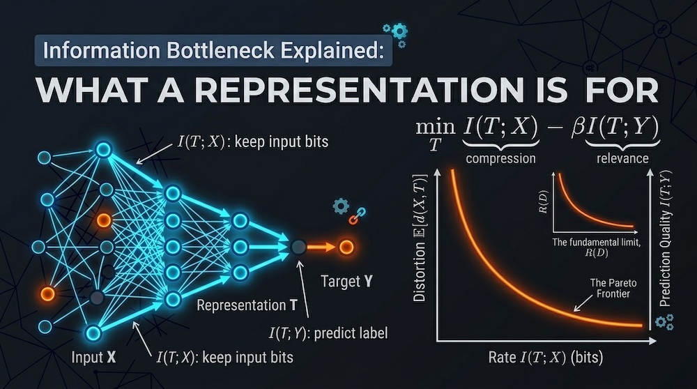
The information bottleneck for practitioners: what it means to keep only the bits that predict, why the binned compression phase in our experiment tracks the activation function rather than learning, why every information-plane number depends on its binning while the exact one for a finite input does not, and how the same equation — not the same explanation, and with β multiplying the opposite term — shows up in a VAE's collapsed latent.
Prerequisites: entropy, cross-entropy, KL divergence and mutual information at the level of this week's other explainer, Information Theory Explained, in particular its §6 on estimator bias. Everything here is a consumer of those four definitions.
Reading path. On a first pass the core is §1 (what the objective asks, in one two-bit table), §2 (what our experiment shows and what it does not), §4 (the same equation inside a VAE — same shape, with on the opposite term) and §5 up to the L1–L4 table. The precision tables and noisy readout in §3, the level-set arithmetic in §4.1 and the codec measurement in §5.2 are deeper reading: they are where the numbers earn their fences, and they can be skipped without losing the argument.
Companion Notebooks
This article pairs with two notebooks. 00_information_theory_from_scratch.ipynb carries the information-plane experiment — two small networks trained to convergence on a task whose input entropy is exactly known, with hand-derived gradients checked against finite differences; the exact of every layer, computed by counting distinct activation vectors with no estimator at all, beside the binned value at six bin counts; and the rate–distortion curves computed with Blahut–Arimoto and verified against their closed forms. 01_entropy_across_the_series.ipynb carries an ELBO level-set experiment showing how the same score can hide different rate–distortion decompositions; it does not demonstrate an optimum or posterior collapse. Both are pure NumPy, CPU-only, and ship fully executed.
Every experiment table and printed block below is reproduced from their output — Python 3.14.5, NumPy 2.5.3, macOS on Accelerate BLAS, float64 throughout, seeds 20260921 and 20260927 fixed in each notebook's first cell — unless the text says otherwise: a few values are derived algebraically from those tables in the prose (the §2.2 shortfall decomposition, the uniform-occupancy references in §3), and the Blahut–Arimoto convergence check in §5 was run separately with the notebook's own function, its script and output kept with this article's review record. The reproducibility paragraph at the end of §3 says which of those numbers travel to another machine (the closed-form checks) and which do not (the trained-network collision counts). A common claim about experiments of this kind is that the mutual information is infinite. Here it is not, and §3 says what it actually is.
1. The question the bottleneck answers
Suppose you want to predict whether a photograph contains a cat. The photograph is a few million numbers. For that task, almost none of them matter: the lighting, the background and the exact pixel values along the cat's left ear carry little about whether there is a cat. Which numbers are nuisance is a fact about the task and the data, not about photographs — the same lighting is the signal in a time-of-day classifier.
So a good representation of the photograph should throw nearly all of it away — and keep precisely the part that predicts the label.
That sentence is the whole idea, and the information bottleneck (Tishby, Pereira & Bialek, 1999; Tishby & Zaslavsky, arXiv:1503.02406) turns it into an objective. Write for the input, for the label, and for your internal representation. You want to solve:
Two terms, pulling opposite ways:
- — the compression term. How many bits about the input does your representation carry? You want this small, holding the next term fixed. A representation that memorises the input has discarded nothing yet — wasteful exactly when some of what it kept is irrelevant to the label.
- — the prediction term. How many bits about the label does it carry? You want this large.
- — the exchange rate between them.
The claim embedded in this is genuinely interesting: a good representation is defined by what it discards. Not by what it stores. This inverts the intuition that a richer feature vector is a better one. But read it exactly: a good representation is not simply one that remembers less; it is one that preserves what predicts the target while discarding what does not. The objective trades compression against predictive relevance, and it does not, by itself, prove a generalisation theorem — §2.1 says what our experiment can and cannot measure about that.
There is a clean extreme case worth holding onto, and it has to be stated carefully because the lazy version is false. Set : you have kept everything, so is as large as it can possibly be — and is as large as it can be. Whether that is a bad representation depends on how much of was not about . If every bit of the input is task-relevant — a fair bit, , so — there is nothing to compress away, and for any the objective's value is as low as any can reach: keeping everything is then optimal, not useless. Keeping the input becomes inefficient only when some of what it retains is irrelevant to the target, and the compression term prices exactly that part.
1.1 The objective in one table
Before any network, the smallest example that has something to discard. Let be a fair bit and an independent fair bit — a nuisance — and let the input be the pair , so bits and bit. Four deterministic representations, with their two terms (for a deterministic on a uniform finite input, — the same lemma §3 leans on):
| representation | at | ||
|---|---|---|---|
| keep everything, | 2 bits | 1 bit | 0 |
| keep the label bit, | 1 bit | 1 bit | −1 |
| keep the nuisance, | 1 bit | 0 bits | 1 |
| keep nothing, constant | 0 bits | 0 bits | 0 |
At the winner is : preserve the bit that predicts and discard the bit that does not. Keeping everything ties with keeping nothing, because the second bit costs one unit of rate and buys no relevance — and if were instead a second copy of , then , keeping everything would cost nothing extra, and and would tie at — they are the same representation up to relabelling. That is the information bottleneck in one table. What the rest of this article adds is the question of whether a trained network behaves as though it were optimising it, which turns out to be a much harder question than the table suggests.
2. The famous claim: two phases of training
The result that made this framework widely discussed (Shwartz-Ziv & Tishby, arXiv:1703.00810) is an empirical observation about what happens when you plot training in the information plane — on one axis, on the other, one point per layer per epoch.
The claim is that training has two distinct phases:
- Fitting — short. Both quantities rise. The network learns to predict.
- Compression — long. stays flat while falls. The network keeps its accuracy while progressively forgetting the input.
If real, that is a striking picture: most of training is not learning, it is discarding. And it would suggest that generalisation comes from the compression phase.
It is also a claim you should not accept on the strength of a plot, so we measured it.
2.1 Our setup, and why it is built this way
Mutual information is hard to estimate reliably from high-dimensional data because the joint distribution it is defined on — — is usually unknown; knowing on its own is not the prerequisite, and for a deterministic representation of a discrete source the quantity reduces to . So the notebook uses a task whose complete input distribution is known: all 4,096 distinct 12-bit patterns, each appearing with probability . That gives both an exact ceiling, bits, and an exact by enumerating the deterministic representations.
X: (4096, 12)  (all 4096 patterns, each with probability 2^-12)
Y balance: 0.5000 H(Y) = 1.000000 bitsbits exactly, bit exactly. No estimation error in the ground truth: the input distribution and every deterministic count in this article are known exactly, so those numbers are about the network rather than about our sampling. The one exception is §3's noisy readout, a stochastic channel whose information is numerically integrated and reported with an error bar.
Two networks with the same architecture (12 → 10 → 7 → 5 → 4 → 3 → 2), the same task, the same full-batch schedule (4,000 epochs at learning rate 0.6) and the same seed, differing in the activation function — one tanh, one ReLU — and in two things that follow from it: the initialisation gain (1 for tanh, for ReLU — the He correction without which the ReLU funnel never leaves chance) and the range the 30-level readout quantiser spans (a fixed for tanh; of the layer's own activations for ReLU). So this is a matched reproduction of a qualitative phenomenon, not a one-factor ablation: what the comparison isolates is tanh-with-its-standard-recipe against ReLU-with-its-standard-recipe, and the Saxe et al. conclusion below rests on their broader study, not on this pair alone. Gradients are derived by hand and verified against finite differences before any conclusion is drawn:
 tanh: 6 layers checked, all within 1e-5 relative error
 relu: 6 layers checked, all within 1e-5 relative error
And both actually learned the task, which matters — otherwise any difference between them is a difference in training success, not in representation:
 tanh: final epoch 4000  loss 0.00008 nats  train accuracy 1.0000
 relu: final epoch 4000  loss 0.03921 nats  train accuracy 0.9890
One limit of the design, stated before the results. Because the training set is the entire finite input support — all 4,096 patterns — there are no held-out inputs within this population, and the accuracies above are training accuracies. The experiment measures information dynamics and training fit, not generalisation to unseen inputs: it is built to test how the information-plane measurements behave, not whether compression improves held-out accuracy, and nothing below should be read as evidence on that second question.
2.2 What we found
One thing before the table, which §3 will make precise: every value in it is the entropy of the activation vector after each unit has been quantised to 30 levels. The notebook labels the column I(T;X) because that is what the information-plane literature calls it. What it actually is, is for the 30-level quantiser — and because the notebook enumerates the whole input set, that is an exact number for its own readout, with no sampling error and no estimator. It is not an estimate of anything, and in particular not of the float64 layer's , which §3 counts separately, with no bins, and which is larger: always, and a different gives a different exact number. (Uniform on four values, , : bits and bit, both exact, two channels.) Read the table as "how much of the input's identity survives a 30-level quantisation of each unit", which is a statement about how tightly the layer clusters its activations.
Per-layer I(T;X): value at its peak, and at the end of training (30 bins)
  act  layer  peak I(T;X)     final    change
 tanh      1      12.0000   11.9893   -0.0107
 tanh      2      12.0000    8.4147   -3.5853
 tanh      3      11.8529    3.6580   -8.1948
 tanh      4       8.9857    2.0854   -6.9003
 tanh      5       7.9751    1.5376   -6.4375
 relu      1      11.7029    8.3856   -3.3173
 relu      2       8.0739    5.6741   -2.3998
 relu      3       8.0004    4.9885   -3.0119
 relu      4       5.2580    5.1328   -0.1252
 relu      5       3.4599    3.3971   -0.0628
In the tanh network, the binned quantity falls, and it falls a lot. Layer 3 rises to 11.85 and then sheds 8.19 while accuracy climbs to a perfect 1.0000. The deepest layer finishes at 1.54, the lowest figure in the table. Resist reading that 1.54 against the 1 bit the task requires: §3 shows the same measurement running from 1.21 to 2.34 as the binning is refined, so how near it lands to is a property of the 30 bins rather than a finding about the network. Layer 1 barely moves (−0.01), layer 5 moves heavily. That is the shape the information-bottleneck story predicts. Whether it is the thing the story describes is the question §3 answers, and the answer is narrower than the shape suggests.
In the ReLU network the late-layer pattern is much weaker — not absent. Layers 4 and 5 shed 0.13 and 0.06, essentially nothing, while layers 1–3 shed 3.32, 2.40 and 3.01 bits — real peak-to-final decreases, concentrated in the early layers, which is the opposite pattern from tanh's.
The ReLU rows carry one more caveat, and it is about the ruler rather than the network. The tanh readout spans a fixed , so its trajectory compares one quantiser across epochs. The ReLU readout spans of the layer's current activations, recalibrated at every measurement, so a ReLU trajectory is with both the representation and the quantiser moving with the epoch : a peak-to-final change there can be the activations moving, the bin edges moving, or both. Each value is still exact for its own readout; what is limited is the reading of their changes over training. A fixed-range ReLU trajectory would be the robustness check, and we have not run it.
What this table establishes is qualitative, and it is narrower than "robust to binning": at the 30-bin readout, the tanh network's binned quantity falls steeply in its late layers during training and the ReLU network's late layers change little. The bin-count sweep in §3 is a final-checkpoint measurement of the deepest layer — at every bin count we tested, tanh ends lower than ReLU — and the trajectories were recorded at 30 bins only, so we have not established that the full training curves keep the same shape at every resolution. The bit values are exact findings for their specified quantised readouts, not intrinsic information values of the unquantised representations. Keep that distinction in hand for the rest of the section.
Why the final information shortfall has two components
Before drawing any conclusion from that table, notice that it has three columns and most discussions of the information plane quote only one of them. Read peak and final together, because a deep layer's final distance from the 12-bit ceiling is not a single phenomenon, and the change column reports only part of it.
In the tanh network, layers 1 and 2 both peak at the full 12.0000 bits — they held the entire input at some point in training. Layer 3 peaks at 11.85, essentially all of it. But layers 4 and 5 peak at 8.99 and 7.98: they did reach those observed peaks, and what they never approached was the 12-bit ceiling under this quantiser. Those two layers never displayed the whole input at any probe.
So separate the two components, because the table's own definition puts only one of them in the change column. That column is , the peak-to-final decrease and nothing else. What combines the two effects is the final shortfall from the 12-bit input entropy:
For the tanh network's two deepest layers — every figure at the 30-bin readout, not the exact float64 representation. The middle column is the printed change entry with its sign flipped, : the table above prints layer 5 as , and the same quantity appears here as a loss of 6.4375, so neither table has the sign wrong.
| layer | never resolved at peak, | peak-to-final loss, | final shortfall, |
|---|---|---|---|
| 4 | 3.0143 bits | 6.9003 bits | 9.9146 bits |
| 5 | 4.0249 bits | 6.4375 bits | 10.4624 bits |
The two components are different things:
- Binned bits acquired and then shed — the magnitude of the
changecolumn, whose printed entries carry the minus sign. Layer 3 is the clean case: up to 11.85, down to 3.66, a loss of 8.19 bits while training accuracy climbed to 1.0000. This is the compression phase as the plot describes it — a layer whose activations were once spread widely enough for a 30-level quantiser to separate the inputs, and then were not. Hold the stronger reading until §3, which counts the same layer exactly: it maps every input to its own vector at every probe epoch, so what it stopped doing is spreading, not carrying. - Binned bits never acquired — the first term, which the
changecolumn does not see. Layer 5 finishes at 1.54, the lowest figure in the table, but its binned peak was only 7.98: under this quantiser, four of the twelve input bits never reached it. Read that as a statement about the readout too. §3's per-checkpoint count finds the same layer at 12.0000 exact bits at every probe, so the input did reach it — packed into a cloud the quantiser could not resolve. An upstream layer that genuinely lost bits would cap everything below it, which is the data-processing inequality operating inside your own network; here no tanh layer did.
Both are compression in the sense that the deep layer's quantised readout ends up carrying few bits about the input. They are different as geometric facts — the first layer clustered during training, the second was clustered from early on — and neither is information loss in the exact sense.
The same reading changes the ReLU story too. ReLU's layer 5 peaks at 3.46 bits against tanh's 7.98 — so its small final value of 3.40 is not restraint; under this quantiser it never read out much, and here §3's exact count agrees, because that layer genuinely starts training with 227 distinct vectors and 67% of its units dead. Quoting only its change (−0.06, "no compression") and only tanh's change (−6.44, "lots of compression") gets the ordering of final values exactly backwards: tanh ends at 1.54 and ReLU at 3.40.
Whenever you see an information-plane trajectory, ask how high the curve went before it came down — and then ask what readout it was measured through. A binned curve that never rose is not compressing; under that quantiser it was clustered from the start, which can mean a starved layer or a tightly packed one, and only an exact count or a stated noise channel (§3) tells you which. For our tanh layer 5 it was the second; for our ReLU layer 5 it was the first.
This is the Saxe et al. (ICLR 2018) objection, reproduced. The binned compression phase is a property of the saturating nonlinearity, not a universal law of learning. A tanh unit has flat regions; pushing activations into them clusters distinct inputs onto nearly indistinguishable outputs, which a 30-level quantiser then merges. ReLU is unbounded above and does not saturate the same way, so that clustering mechanism is much weaker in its late layers; what its early layers shed under the same quantiser is a different, smaller movement, and the dead units in §2.3 are a third thing again.
The status of the claim, stated rather than implied. One notebook with one pair of networks is an illustration, and the field's position should be on the page. The fitting-then-compression story is not the current default explanation of deep training. Outside saturating nonlinearities the compression phase is generally not observed (Saxe et al.); when noise is injected so that is finite and genuinely estimable, the measured quantity tracks geometric clustering of the representations rather than any information-theoretic phase (Goldfeld et al., 2019); and the live explanatory alternatives — neural collapse of the last-layer features, grokking, and geometric accounts of representation learning — need no information-theoretic phase at all. The information bottleneck as an objective is alive and useful, and §4 is where it earns its keep. The information bottleneck as a theory of SGD is contested, and our experiment does not settle it. It was not designed to.
2.3 A blunter mechanism hiding in the same plot
There is a second thing happening in the ReLU network that no elegant theory explains:
Permanently dead ReLU units by layer: ['0%', '0%', '40%', '25%', '67%']67% of the deepest layer's units output zero for every one of the 4,096 inputs. A unit with a constant output carries no bits about anything — this is information destruction in the most literal form available, and it needs no bin count and no estimator to see. It is a statement in the network's own neuron coordinates — the ones the next layer actually reads — and not a coordinate-free fact about the information: §3 gives the two-line example in which an invertible change of coordinates takes a layer from half its units dead to none, with the mutual information untouched. Lead with it — and do not let it stand in for the loss, which §3 counts separately.
Dead units are one mechanism by which a layer can collapse distinct inputs onto identical representations, so part of what an information-plane plot displays as "compression" can be units dying — capacity being lost, not a representation learning to be selective — and that is worth ruling out before you read a falling curve as evidence of an elegant learning dynamic. Rule it out here, though, and it is not the explanation: the tanh network, whose binned curves fall furthest, has no dead units at all, and §3's per-checkpoint table finds the ReLU network's dead units already present at the first probe, with that layer's exact information rising afterwards. In this experiment dead units help explain some ReLU collisions; they explain nothing about tanh's downward binned trajectory. And §3 will show that the ReLU network's deep layers are the only places in the experiment where the exact mutual information — not the binned one — falls below the ceiling, and that the dead units explain some of that loss and not all of it.
3. The objection you must internalise before quoting any of these numbers
Everything above came with "(30 bins)" attached, and that parenthetical is doing more work than it appears to.
The information-plane literature computes for continuous activations by discretising them into bins. That is one measurement method, not a necessity — for this experiment, counting distinct activation vectors gives the exact answer with no bins at all, which is what the second table in this section does — but start with the bins, because they are what §2 reported. We ran the identical final-epoch measurement of the deepest layer at several bin counts:
Final-epoch I(T;X) of the deepest hidden layer, as a function of bin count
  bins       tanh       relu
     8     1.2124     2.1748
    16     1.3296     2.8675
    30     1.5376     3.3971
    60     1.6883     3.9717
   120     1.7661     4.5322
   256     2.3442     5.1362

For reference, H(X) = 12.0000 bits — the hard ceiling on I(T;X).
The tanh figure roughly doubles from 8 bins to 256. The ReLU figure more than doubles. And these numbers generally tend toward a limit as the bins are refined — not necessarily upward at every bin count, because equal-width partitions at different counts are not nested in one another, so a value can fluctuate as the edges move, though fine enough bins eventually separate every distinct activation vector of this finite set — and the usual account of that limit is wrong for this experiment. It says: for a deterministic network on continuous activations is a function of , so diverges as the discretisation is refined, and the true mutual information is infinite. That is true for a continuous input distribution when the representation keeps a continuous component — for has infinite mutual information with . It is not true of continuous inputs as such: a deterministic representation with a discrete output has finite mutual information however continuous the input — on the same gives bit, and a constant gives 0. The input distribution alone does not determine the answer; the representation's output does. And it is false for this experiment, and the whole point of the experiment was that is exactly known.
What the exact quantity is, for this experiment. has finite support — 4,096 equiprobable points — and is a deterministic function of . So bits, exactly, where is the activation vector at floating-point precision. There is no infinity anywhere in this setup. And needs no estimator at all: count the distinct activation vectors over the 4,096 inputs and take the entropy of their empirical distribution.
The notebook does that, for every layer of both networks at the end of training, and puts the 30-bin value beside it, with two binning-free measures of the layer's geometry — the effective rank of its activation covariance (the exponential of the entropy of its normalised eigenvalues) and the fraction of units that are constant on the whole input set:
Exact I(X;T) = H(T) at float precision, final epoch, vs the 30-bin value
  act  layer  width  distinct  H(T) exact   30-bin  eff.rank  const units
 tanh      1     10      4096     12.0000  11.9893     2.441          0%
 tanh      2      7      4096     12.0000   8.4147     1.186          0%
 tanh      3      5      4096     12.0000   3.6580     1.053          0%
 tanh      4      4      4096     12.0000   2.0854     1.030          0%
 tanh      5      3      4096     12.0000   1.5376     1.026          0%
 relu      1     10      4096     12.0000   8.3856     1.717          0%
 relu      2     7       4096     12.0000   5.6741     1.572          0%
 relu      3      5      4065     11.9609   4.9885     1.313         40%
 relu      4      4      4065     11.9609   5.1328     1.537         25%
 relu      5      3      2271      7.2237   3.3971     1.000         67%

7 of 10 layers keep all 4,096 inputs distinct (H(T) = 12 bits exactly).
Every count in that table is at float64, the precision the layers were computed in, and it is a readout statement rather than a weights statement: the cast table further down repeats the count at float32 and float16 for the same trained weights, and the deepest tanh layer's 4,096 distinct vectors become 445 — 4.29 bits, which on a support of 445 means a heavily skewed occupancy, since 445 equally filled vectors would be bits and 4.29 bits is only equiprobable vectors' worth — once the readout is float16. Those two numbers are not one fact, and the second does not say which vectors hold the inputs: is the number of equally probable vectors that would carry the same entropy, an effective support size, not a count of vectors that capture most of the 4,096 inputs. An occupancy with one vector holding 2,541 inputs and the other 444 holding three or four each also has 4.29 bits, and its twenty fullest vectors cover only 64% of the inputs. Reading the mass needs the occupancy counts or a cumulative-mass curve, which the notebook does not print.
Read the tanh rows first, because they overturn the headline. Every tanh layer carries all 12 bits about the input, exactly, at the end of training. Layer 3 — the one whose 30-bin value fell from 11.85 to 3.66, the "8.19 bits of compression" — maps every one of the 4,096 inputs to its own distinct activation vector. It has compressed nothing, in the information-theoretic sense. What happened is visible in the effective-rank column: the layer's activations collapsed onto essentially one direction (effective rank 1.05 across five units), tightly clustered, so that a 30-level quantiser merges most of them. The binned curve measured the layer clustering its activations as it saturated. That is a real and interesting geometric event. It is not information loss, and calling it "compression" in bits was the error.
The ReLU rows tell the opposite story, and it is the one worth quoting. ReLU layer 5 genuinely loses information: 2,271 distinct vectors, bits of a possible 12. What loses the bits is collisions — two inputs mapped to the same activation vector — and the last column is where they happened, not by itself why. Dead units are a route to collisions, not a proof of them: a unit that is constant on every input carries zero bits on its own, but a layer with two dead units and one live unit that happens to take a distinct value on every input still carries all twelve (take — one neuron, 4,096 distinct outputs), so a dead-unit count neither proves nor quantifies a layer's loss. Here the two coincide: layer 5, with 67% dead units and a single live rectifier, clips many inputs onto the same output and keeps 2,271 distinct vectors; layers 3 and 4, with 40% and 25% dead units, each merge a handful (11.96 bits); and the per-checkpoint table below shows where the two counts agree and where they do not: layer 5's dead units and its collisions are both present at the first probe epoch, while layer 3 collides inputs at epoch 1 with 0% dead units and grows its first dead unit only at probe epoch 3,644. A rectifier does not have to be dead on every input to merge two of them — it only has to be off on the inputs where they differ. That is the measured relationship, and it is a relationship between two counts, not a theorem that one causes the other. The ReLU network is not "failing to compress"; its deep layers are colliding inputs.
So the information plane of this experiment, measured exactly, is almost a point that does not move: twelve bits at every tanh layer, twelve at the first two ReLU layers, and a genuine drop only in the ReLU layers where inputs collided — in layer 5 where units died, and in layers 3 and 4 without any dead unit at the epoch the collisions appeared. Every finite number in the binned tables — and in every information-plane paper that bins activations — is therefore a property of the quantiser as much as of the network, and it measures how tightly activations cluster (Goldfeld et al., 2019 make this precise: binned "compression" tracks geometric clustering of the representation).
This does not make the binned measurement useless, and the distinction matters:
- An absolute binned value of in bits, reported without its binning scheme, is not a quantity. Treat it the way you would treat a distance reported without units. The exact value, where it is computable, is the quantity.
- A comparison can still be sound if both sides are binned identically. Our tanh-versus-ReLU ordering holds at every bin count we tried — tanh ends lower than ReLU at 8, 16, 30, 60, 120 and 256 bins. The ordering is stable even though the values are not. But notice what the ordering means now that the exact column exists: tanh reads lower because it clusters harder, while carrying more exact information than the ReLU layer it is being compared with. The ordering is a finding about geometry.
- Binning-free measures exist, and they should lead — but bin-free is not choice-free. The dead-unit fraction and the effective rank in the table above need no bin count. Effective rank is a property of the covariance spectrum, though, so it moves under a rescaling of coordinates that leaves the information untouched: take with identity covariance, effective rank 2, and read the same layer as — an invertible map, so exactly, while the eigenvalues become 10,000 and 1 and the effective rank falls to 1.001. It is a geometry measure in whatever units the layer happens to use, which is the same reason the absolute and RMS-normalised noisy readouts below can disagree; and the dead-unit fraction is not coordinate-free either. Take a two-unit layer with non-constant: half its units are dead. Apply the invertible map and : no unit is dead, and exactly. The dead-unit fraction is a precise architectural diagnostic in the coordinates the next layer reads — which is why it is worth reporting — not an invariant of the representation's information. The information a representation preserves and the geometric or architectural statistics used to describe it are different objects; that is the lesson of this whole section. For a continuous input and a representation with a continuous component, where the exact value really would be infinite, the honest designs are to inject noise of a stated variance so that is finite and estimable with a stated bound, or to report the geometry directly. The companion notebook runs that noisy leg on these same networks, with Gaussian noise of standard deviation 0.01, 0.1 and 0.5 on the activations — the first about a hundredth of the activation RMS — computed as a Monte Carlo expectation over the known 4,096-component mixture with a stratified standard error, no bins and no learned estimator (the density is exact; the integral is Monte Carlo, which is why only these numbers carry error bars). At tanh layer 3 reads out at 4.2 bits of its exact 12 and ReLU layer 5 at 5.6 bits of its exact 7.22 (at and : 2.08 and 1.24 bits against 3.81 and 2.48), so the ordering between the two networks flips the moment a readout channel is named. The same noise expressed as a fraction of each layer's own RMS — the comparison that survives a rescaling a downstream layer could absorb for free — keeps that flip in the three deepest layers (ReLU 7.66, 7.23 and 4.58 bits against tanh 4.27, 2.48 and 1.61 at 1% relative noise) and reverses it in layer 2, so in the layers where the tanh network has collapsed onto one direction the difference is geometry, and one layer up it was scale. Three noise levels are three points, not a curve; the orderings are findings about these two channels on these two networks, not an architectural ranking independent of readout noise.
One distinction to carry, because the companion piece and this one use the words "mutual-information estimate" in different settings and the difference is the whole of this section:
| situation | what can go wrong |
|---|---|
| full distribution known, deterministic quantiser — this experiment's 4,096-input count, binned or exact | no sampling error at all; the binned value is exact for its quantiser, and a different quantiser gives a different exact number |
| finite sample, histogram plug-in — the companion piece's §6 | sampling variability and a bias whose sign depends on the regime |
| continuous representation plus Gaussian noise of a stated variance — the noisy readout above | a well-defined channel quantity; here the density is exact and only the Monte Carlo integral carries an error bar |
| learned neural estimator (MINE and its relatives) | estimation and optimisation error, with a bound or a variance limitation |
Nothing in this article's binned tables carries a sampling error bar, and nothing in them should be read as a quantity independent of the ruler.
The precision is part of the measurement, so the notebook varies it. Every array in the notebook is float64, so "distinct" in the table above means distinct as float64, and the 12.0000 is a float64 number. A consumer that reads the layer at lower precision reads a different map, and the notebook casts the same float64 activations — same weights, same forward pass — to float32 and to float16 before counting. These are readout casts, not networks trained at lower precision:
Readout-precision ablation: distinct activation vectors and H(T) [bits] when the float64 activations
are CAST to a narrower dtype before counting (same trained weights; the cast is at the readout only).
  act  layer |            float64 |       float32 cast |       float16 cast
 tanh      1 |   4096    12.0000 |   4096    12.0000 |   4096    12.0000
 tanh      2 |   4096    12.0000 |   4096    12.0000 |   4095    11.9995
 tanh      3 |   4096    12.0000 |   4096    12.0000 |   2990    11.1031
 tanh      4 |   4096    12.0000 |   4096    12.0000 |   1234     8.1140
 tanh      5 |   4096    12.0000 |   4090    11.9971 |    445     4.2910
 relu      1 |   4096    12.0000 |   4096    12.0000 |   4095    11.9995
 relu      2 |   4096    12.0000 |   4096    12.0000 |   3630    11.7501
 relu      3 |   4065    11.9609 |   4065    11.9609 |   3565    11.6983
 relu      4 |   4065    11.9609 |   4065    11.9609 |   3154    11.4652
 relu      5 |   2271     7.2237 |   2271     7.2237 |   1473     6.7696
The float32 cast merges 6 of the 4,096 inputs in tanh layer 5 and none elsewhere in that network; the float16 cast leaves 445 distinct vectors at the deepest tanh layer — 4.29 bits against the 12.0000 that float64 reports, and well below the 8.80 that 445 evenly filled vectors would give, so the surviving vectors are unevenly filled — in the layer whose activations the noisy readout found packed a hundredth of their RMS apart. ReLU layer 5 goes from 2,271 distinct vectors at float64 and float32 to 1,473 at float16 (6.77 bits). For a deterministic map on a finite input set is exact at every precision; what the cast changes is the map whose entropy is being counted. Quote the 12.0000 as a float64 number, and do not read it as what an FP32 or FP16 consumer of the layer would see.
A final-epoch table cannot show that the exact plane was static — the compression claim is about a trajectory — so the notebook records the exact collision count and the dead-unit fraction at seven probe epochs of the same training pass, from the same forward pass as the binned value, and asserts that the final probe equals a fresh forward pass of the final weights. Every tanh layer holds 4,096 distinct vectors — 12.0000 bits — at all seven probes, epochs 1, 2, 5, 10, 20, 50 and 4,000. Seven probes do not rule out an excursion between them, but a compression phase invisible at all seven is not the one the two-phase story describes, and the binned curve's steep descent in §2.2 is entirely the ruler. The ReLU rows run against the compression story:
relu
 epoch     acc |  L3 H(T)  dead |  L4 H(T)  dead |  L5 H(T)  dead | L5 distinct
     1  0.4880 |  11.7914    0% |  11.7554   25% |   0.7395   67% |         227
     2  0.4871 |  11.7914    0% |  11.7554   25% |   0.7232   67% |         222
     5  0.4883 |  11.7900    0% |  11.7494   25% |   0.6710   67% |         206
    10  0.4910 |  11.7900    0% |  11.7413   25% |   0.5991   67% |         184
    20  0.4919 |  11.7900    0% |  11.7347   25% |   0.5305   67% |         163
    50  0.4932 |  11.7927    0% |  11.6916   25% |   0.3343   67% |         103
  4000  0.9890 |  11.9609   40% |  11.9609   25% |   7.2237   67% |        2271
  layer 3: first collision at probe epoch 1, first dead unit at probe epoch 3644
  layer 5: first collision at probe epoch 1, first dead unit at probe epoch 1
Layer 5's 67% dead units are dead at the first probe, and its exact information rises from 0.74 bits (227 distinct vectors) at epoch 1 to 7.22 bits (2,271) at epoch 4,000: two of its three units never fire on any input, and training spent 4,000 epochs teaching the one live rectifier to separate inputs it had initially merged. Layer 3 collides inputs at epoch 1 with 0% dead units and grows its first dead unit only at probe epoch 3,644, by which time its collision count has fallen. In this experiment the exact of the ReLU network goes up wherever it moves at all, and every exact loss is a collision present from initialisation.
That is the general shape of honest work with these quantities: compute the exact quantity when you can, trust the comparisons you controlled, distrust the absolute binned numbers, and always say what your denominator was.
Reproducibility scope, stated once. Within the environment named at the top a re-execution reproduces every number. Across environments the scope is narrower, and the notebooks say so: an independent re-execution on Linux (Python 3.13.5, NumPy 2.3.5), reported to us during review, reproduced every closed-form check in the first notebook and every number in the second, and moved the trained-network numbers — the ReLU network reached a final accuracy of 0.9946 rather than 0.9890, with 4,017 distinct vectors at layer 3 rather than 4,065 and 2,252 at layer 5 rather than 2,271, from the same seed. Nothing is wrong with either run: 4,000 epochs of full-batch gradient descent amplify last-bit differences between two BLAS implementations into different weights, and a count of exact floating-point collisions is the most sensitive statistic one could build on them. What is portable is the set of findings this section states, not the third digit of a collision count, and the trained weights ship beside the notebook as nb00_trained_params.npz so the representation can be read without retraining it.
Recent work reformulates the bottleneck through synergy — information obtainable only through the joint processing of features, measured with the average interaction information of each feature with the rest — and reports empirical results across architectures, including ReLU networks where the binned plane shows nothing (A Generalized Information Bottleneck Theory of Deep Learning, arXiv:2509.26327). Its theorem relating the two objectives is conditional, and the conditions belong beside it: under perfect training accuracy and a deterministic network, so that the output can be identified with the label, the original IB objective is upper-bounded by the generalised one. For a network that has not fit its training set, or that is stochastic, the bound is not asserted. Read it as a proposed generalisation with a conditional relationship to IB and an empirical case — the width the paper itself claims.
4. The same equation, wearing a VAE
Here is where the bottleneck stops being a lens for analysing networks and starts being something you have already trained.
Write the negative ELBO — the thing a variational autoencoder minimises:
Now rename the two terms. The reconstruction error is distortion — how badly you recover the input. Averaged over inputs, the KL term is rate, and the claim that it is a rate has a one-line proof: let be the aggregate posterior, add and subtract inside the expectation, and
the mutual information between input and latent under the encoder plus a non-negative gap (Hoffman & Johnson, 2016; Alemi et al., Fixing a Broken ELBO, 2018). So the average rate is an upper bound on the information the latent carries about the input, tight when the aggregate posterior matches the prior. Averaged over data:
The negative ELBO splits exactly into a distortion and an upper bound on rate. One warning before the symbol appears: when §4.2 turns that price into a dial, , the multiplies the rate — the opposite term from §1's , where it multiplies relevance. Same shape, opposite placement, and "large " is not an instruction until you have said which term it sits on. That has the form of a rate–distortion Lagrangian with the price of a bit fixed at 1 — with an upper bound rather than Shannon's minimum over all channels, and the two meeting only where the encoder family contains the optimum, as the linear-Gaussian family below does at exactly one . In the trend tutorial's grading this is L2, a variational correspondence with every term defined, and it is the place where the "it's rate–distortion" reading is earned rather than asserted — at exactly that width. It is the same two-term structure as the bottleneck: spend bits, reduce error, and trade one against the other. The level-set observation below is Alemi et al.'s, not a discovery of this series, and the variational treatment that made the bottleneck itself trainable at scale is Deep VIB (arXiv:1612.00410). They share a variational trade-off structure, with different prediction targets.
Seeing that immediately explains a failure mode that otherwise looks like a bug.
4.1 Posterior collapse, explained properly
Posterior collapse broadly describes a VAE failing to use its latent as intended, and it is not one event. It may appear as negligible mutual information between input and latent, as a near-zero KL rate, or as a decoder that ignores and degenerates into an unconditional generator. The three are related and not equivalent — an encoder whose posterior is the same for every input carries nothing about () yet can pay a non-zero KL if that posterior differs from the prior, and a decoder can ignore while the encoder's posterior still moves with — and which one occurred decides the remedy, which is what the procedure in §4.2 measures. It is usually described as a training pathology to be worked around with KL annealing, warm-up schedules, or architectural constraints.
Both the objective and optimization can contribute. We first separate a score ambiguity from an actual collapsed optimum.
First, the vocabulary. Three encoders on the same task:
                     encoder  rate R [bits]  distortion D [bits]   -ELBO = R+D
       collapsed (a=0, s2=1)         0.0000              14.8131       14.8131
    balanced (a=0.6, s2=0.3)         0.6492               3.0984        3.7476
 high-rate (a=0.95, s2=0.05)         2.1918               0.0453        2.2371
These three have different ELBOs, so they are not yet the problem — they just establish the axes. The zero-rate encoder has a much worse negative ELBO here; the high-rate encoder reduces the negative log-density term. Rate is a bound on mutual information, and a small continuous negative log-density is not a statement of zero squared reconstruction error.
The problem appears along a level set — the set of encoders with the same objective value:
Encoders whose -ELBO equals 2.3131 bits to within 0.002:
  count                : 725
  rate R spans         : 1.2578 to 2.3398 bits  (a spread of 1.0820 bits)
  distortion D spans   : -0.0251 to 1.0571 bits
725 encoders lie within 0.002 bits of one score, with rates from 1.26 to 2.34 bits. "Near" means that tolerance, and the band is read off a grid: 1,200 values of on by 900 values of on — 1,080,000 encoders — with the level, 2.3131 bits, taken as the 4th percentile of the objective over that grid, a representative achievable score rather than a special one. The band contains no zero-rate solution and is not a set of minima: these 725 encoders are not stationary points and not where an optimiser ends up, and for a smooth objective in two parameters a curve of near-equal values is unremarkable. Equal scores do not imply a zero gradient or determine where optimisation converges. For the fixed decoder in this experiment the exact posterior , minimises the negative ELBO at 2.1158 bits, 0.2 bits below the band, and the gradient on the band is non-zero; the collapsed encoder above is 12.7 bits worse.
One detail in that output deserves an explanation rather than a silent pass, because it looks like an error: the distortion column starts at −0.0251 bits. A negative distortion sounds impossible, and it would be if this were a count of bits. It is not. Distortion here is an expected negative log conditional density, a continuous cross-entropy term — and differential entropies can be negative whenever the density is concentrated into a region narrower than one unit of the coordinate you measured in. The rate , being a KL divergence, is genuinely non-negative; the distortion is not, and their sum is still the quantity the optimiser sees. Nothing is broken. But it is a good reminder that "bits" in the continuous setting is a unit of comparison rather than a count, which is the same caution §3 attached to and the same reason you should never read one of these numbers without knowing which kind it is.
The experiment demonstrates ambiguity in a scalar score, not posterior collapse. With other decoder families, collapsed solutions can be favored or competitive; optimization can also be responsible. Diagnose the rate, decoder and training dynamics before choosing an intervention.
4.2 β is the price of a bit
If the trouble is that the exchange rate is pinned at 1, then change it. That is the -VAE, minimising — and two things need to be exact before the numbers. First, where the symbol sits, because §1 and this section share it and wire it in opposite directions. In the bottleneck Lagrangian of §1, , multiplies the relevance term: a large spends rate to keep the label. In the -VAE, , multiplies the rate: a large makes bits expensive and the latent goes quiet. Both conventions are standard, and they are opposite dials — a reader who turns the §1 knob to cure the failure below buys more rate. "Large " is not an instruction until you have said which term it sits on. Second, what it changes: changes the objective, not a point on the level set above — it does not select among the 725 encoders, it replaces the function they tie on. Its optima trace a curve:
beta=15.85 lands at R=0.191 bits  (latent nearly unused)
beta=0.06 lands at R=3.731 bits  (latent carrying real information)
Same model family, same data, same ELBO machinery. Only the price of a bit changed.
A roughly 20× swing in latent usage () from the Lagrange multiplier alone — between the two ends of a 200-point sweep of from 0.06 to 15.85, each point minimised over a grid of — with nothing else altered.
Read as a price. Make bits expensive ( large) and the encoder buys almost none — the latent falls quiet. Make bits cheap ( small) and it buys freely — the latent carries real information, at the cost of a less structured prior. Neither is a bug. They are two points on a curve, and is the dial that moves you along it. But the curve traces is not Shannon's . Shannon's function minimises over every conditional with ; a sweep traces the achievable curve of one encoder family and one decoder family, which lies inside the region bounds and touches the boundary only where the family contains the optimum. The running family here is the case where it does — at exactly, where the exact posterior is in the family, the aggregate posterior equals the prior and ; restrict the decoder so the optimum leaves the family and the gap opens (the trend tutorial's §6.1 works the numbers). A sweep explores the family, not the bound.
That shows is a lever on rate. It does not show that is the lever, and the common advice — "if your latent is quiet, change , not your optimiser" — is stronger than anything above supports. The theorem-level fact about posterior collapse points elsewhere: with a decoder expressive enough to model without , a zero-rate solution is a global optimum of the ELBO (Chen et al., Variational Lossy Autoencoder, 2017; the analysis in Alemi et al.) — not necessarily the only one, since another parametrisation of the same marginal can reach the same ELBO with a nonzero-rate exact posterior. What the theorem says is that nothing in the objective prefers the latent to be used: no optimiser change makes it necessary, and moves you off the bound you were trying to maximise. Collapse can also be a trajectory: the KL term dominates early, the encoder is driven to the prior before the decoder learns to use , and warm-up or free bits avoids a poor local solution. These are different causes with different fixes, and neither the level set nor the sweep can tell you which one you have.
Practical consequence — a procedure, not a prescription. When the latent is quiet:
- Measure before intervening, with three diagnostics kept apart. Per-dimension KL (the rate each dimension spends); the active-units statistic of Burda et al., 2016, with its 0.01 threshold (whether the posterior mean moves with the input at all); and the aggregate-posterior gap — which the decomposition above lets you read as the difference between the rate and the information the latent actually carries. The first is not a count of the second: a dimension with for every carries nothing about the input () and still pays nats of KL against a unit prior. Rate can be spent on being narrower than the prior; information needs the posterior to depend on . The converse failure exists too, and it is the activity statistic that misses it: for a fair bit with and , the posterior mean is zero for both inputs, so and the threshold calls the dimension inactive, yet bits — the two conditionals differ, is informative, and a decoder can use it. Activity is a statement about the posterior mean; information can ride the posterior variance. Report all three columns; none substitutes for another.
- Ask whether the decoder can bypass the latent. If it is autoregressive or otherwise able to model alone, the zero-rate solution may be the optimum, and the fix is to weaken the decoder's access to context or to accept that the latent is doing nothing by design.
- Ask whether the trajectory killed it. Compare against KL warm-up (Bowman et al., 2016) or free bits (Kingma et al., 2016) at the same final objective. If the latent is used under warm-up and not without it, the cause was the path, not the objective.
- Check the approximation. A weak inference network makes a rich latent look expensive; a more capable encoder changes the bound, not just the optimum.
- Sweep — the coefficient on the rate in , not §1's — over several seeds and read the result as a rate–distortion curve rather than a cure: it tells you what the latent can carry at each price and where your run landed on that curve.
Changing is one of those experiments, and often the most informative. It is not a universal repair.
5. The floor underneath all of it
One last piece, because it is what makes "rate versus distortion" a real constraint rather than a metaphor.
Rate–distortion theory asks: if I am only allowed bits per source symbol, what is the least distortion I can possibly achieve? The answer is a curve,
for an i.i.d. source and a per-symbol distortion , and the theorem that goes with it has two halves. Converse: no code at any blocklength achieves distortion at a rate below — the hard bound. Achievability: codes exist that approach , in the limit of long blocks, with vector codes that look nothing like a scalar quantiser. Both halves matter below, because "not achievable in practice" and "unachievable" are different claims.
The notebook computes the curve with the Blahut–Arimoto algorithm (Blahut, 1972; Arimoto, 1972) and checks it against the two cases where the answer is known in closed form, domains attached. For a Bernoulli() source under Hamming distortion, on and beyond that — once you tolerate more error than always guessing the majority symbol produces, you need no bits at all:
Binary source p=0.3, Hamming distortion
       D   R measured    H(p)-H(D) exact    abs err
  0.2689     0.041349           0.041349   0.00e+00
  0.1192     0.354226           0.354226   2.22e-16
  0.0474     0.605931           0.605931   0.00e+00
  0.0000     0.881284           0.881284   1.11e-16
For a Gaussian source of variance under squared error, — zero bits once , because sending the mean already achieves distortion . With and that is :
Gaussian source sigma=1, squared-error distortion (241-point quantised grid)
       D   R measured   0.5*log2(1/D)      diff
  0.9999      0.00092         0.00006  +0.00086
  0.9559      0.03250         0.03250  -0.00001
  0.4688      0.54650         0.54651  -0.00001
  0.2285      1.06472         1.06473  -0.00001
  0.1114      1.58294         1.58295  -0.00001
  0.0543      2.10116         2.10117  -0.00001
  0.0265      2.61938         2.61939  -0.00001
  0.0129      3.13760         3.13761  -0.00001
  0.0063      3.65582         3.65583  -0.00001

mean |difference| = 0.00007 bits over 25 points
An iterative algorithm reproducing closed forms to floating-point precision on the binary case, and to a mean absolute difference of bits across the full 25-point sweep on the harder one. That is the check that makes the rest of the notebook worth trusting.
It is also worth noticing where the Gaussian case is least accurate, because the notebook does not hide it — and worth getting the diagnosis right, because the obvious diagnosis is the wrong one. The table above prints every third of the sweep's 25 points; each of those nine rows agrees to except the first, at , which is off by — nearly two orders of magnitude worse than the rest. The notebook's own printed comment attributes that residual to the 241-point grid, and it is the natural reading. It is not primarily the grid. Near the zero-rate endpoint Blahut–Arimoto converges slowly, and the notebook stops that sweep after 800 iterations while its probability updates are still appreciable. Rerunning the notebook's own function on the same grid at the same , varying only the iteration count:
241-point grid, beta=0.253513 (the printed D=0.9999 row)
  iters  R measured        D  0.5*log2(1/D)        diff
    800   0.0009179   0.9999      0.0000553  +0.0008626
   3200   0.0002311   1.0000      0.0000220  +0.0002091
  10000   0.0000601   1.0000      0.0000129  +0.0000471
  20000   0.0000082   1.0000      0.0000101  -0.0000020
The residual falls by two orders of magnitude with the grid untouched, so most of the was incomplete iterative convergence. What remains at 20,000 iterations, a few parts in , this experiment does not isolate: a fixed-grid sweep cannot say how much of it is residual iteration error, finite-grid error, the truncation of the Gaussian's tails at , or floating point, and a separate grid-refinement study at controlled convergence would be needed to measure the grid's own share. The two causes separate only if you test them separately — check convergence against increasing iteration counts first, which we have done, then refine the grid, which we have not — and they do not separate at all if you look at one number and name the cause you expected. (This check is a separate script rather than a notebook cell — it reruns the notebook's own function and is kept with this article's review record, to ship beside the notebook at its next build; the notebook's own printed comment on this row still names the grid, and the table above is its correction.) A version of this article that quoted only the mean would have reported 0.00007 and been perfectly truthful while concealing the one row that tells you what the limitation is — and quoting the row is not enough either, if you then name the cause you expected.
This is the same discipline §3 asked for, in a friendlier setting: the aggregate is not the result, and a number that is well-behaved on average can be well-behaved because you averaged it.
The reason this matters for representations: your encoder is a lossy compressor, and it is subject to this bound — once you have said what the rate is and what the distortion is. When you choose a latent dimension, a quantisation scheme, or a KL weight, you are choosing a point on a curve that exists whether or not you plotted it. But be exact about how the three objects in this article relate, because "they are all rate–distortion" is true at three different strengths, and the trend tutorial's four labels are the discipline for saying which:
| Level | What it means | What you may conclude |
|---|---|---|
| L1 — exact theorem | The quantities and assumptions match a proven result | An identity or a bound you cannot beat |
| L2 — variational correspondence | The objective has the same optimisation structure, with every term defined | A formal analogy you can compute with |
| L3 — engineering heuristic | A similar resource–quality trade-off appears | Design intuition, to be validated |
| L4 — speculative analogy | A resemblance without a derivation | A hypothesis to test, nothing more |
A codec's curve is the theorem itself — L1. The ELBO is an exact split into a distortion and an upper bound on rate (§4, with its proof), whose rate meets Shannon's only where the family contains the optimum — L2. The bottleneck objective is a Lagrangian of the same shape with a different target — the label rather than the input — and a different notion of rate: L2 when both terms are defined and computed, as Deep VIB does, and no more than L3 when is read off a binned plot, which §3 showed is a property of the ruler. Same shape, three levels of claim; the bound forbids something only at the first two.
5.1 Which components deserve bits
The bound tells you how many bits you need. It does not tell you where to spend them — and for that there is a second classical result which turns out to be the most directly actionable idea in this article.
Take a correlated source and look at its eigenvalue spectrum — the variance carried by each independent direction:
Eigenvalue spectrum of the source (the 'which components deserve bits' ranking):
  9.927  2.949  1.128  0.568  0.341  0.229  0.167  0.129  ...
  top 4 of 16 components hold 91.1% of the variance —
Four of sixteen directions hold 91.1% of the variance. The remaining twelve hold under a tenth of it between them.
For a Gaussian source under squared error, the optimal bit allocation across such components is a reverse water-filling solution: imagine pouring water into a container whose floor height is set by each component's variance. Components below the water level receive zero bits — they are cheaper to discard entirely than to encode badly. Components above it receive bits — the log of the ratio between a component's variance and the water level, not of how far it sticks out above it.
This is the entire reason transform coding works. It is worth being precise about why the optimum is a threshold, because the shape is easily promoted into a law about every budget, and it is not one. The problem is subject to and : a separable convex objective whose marginal value is unbounded as , with a hard cap on each . The KKT conditions equalise marginal value across the components that are interior — — and clamp the rest at their cap, which is the threshold. Change any of those ingredients and the threshold disappears: a proportional-fairness allocation is interior, with every share proportional to its weight; an entropy-regularised allocation is a softmax; any problem whose non-negativity constraints never bind has a smooth interior optimum. So the instruction is not "a good allocation is a threshold". It is: write down your constraint set, and check whether it is the one that produces one.
With that fence, the practical reading. The water level is set by the budget, not by the spectrum alone — for a Gaussian source, exactly; for your encoder, as an analogy that holds to the extent that your rate is a rate and your distortion is squared error. For this problem — reconstruct the Gaussian source above under squared error — the first four directions hold 91.1% of the variance, so a four-dimensional projection preserves most of the source's energy and a two-dimensional one discards a component that was genuinely carrying variance. Whether a rate–distortion-optimal code assigns bits to four, fewer, or all sixteen components depends on the distortion you permit: every component with receives bits, the rest receive none, and at a distortion small enough that falls below the smallest eigenvalue all sixteen are active. Reverse water-filling names the active components only after the budget is named. And a latent dimension is not a fixed number of coded bits — dimensionality caps how many components can be active, rate says how finely each is coded, and the two are different constraints, which is why the §4.2 sweep moved the rate 20× inside one latent. That is a statement about compression for reconstruction, and it does not transfer to prediction, because variance is not relevance. Let with of enormous variance and independent of the label, and the sign of a low-variance : water-filling, like PCA, spends its bits on , while the bottleneck objective of §1 keeps and discards entirely. The eigenvalue ranking says which components deserve bits for reconstructing ; which deserve bits for predicting is the question the bottleneck was built to ask, and the two rankings can be opposite.
5.2 Real encoders do not reach the bound, by a predictable amount
One more measurement, because it keeps the bound honest. A practical quantiser does not achieve — it loses roughly a quarter of a bit per sample to the geometry of the lattice it quantises onto rather than to any shortcoming you could engineer away. This is the space-filling loss: a cubic cell is a worse shape than the optimal one, and theory puts the penalty for an entropy-coded uniform scalar quantiser at bits per sample in the high-resolution limit — fine quantisation of a smooth density (Gish & Pierce, 1968). Three claims live here and they are not the same claim: Shannon's bound, which no code at any blocklength beats; its asymptotic achievability by long vector codes; and the gap of one finite codec, which is what the notebook measures.
The notebook builds the quantiser half of a codec on a correlated Gaussian source (, AR(1) with , 200,000 samples) — a KLT, then a uniform scalar quantiser — and charges itself the sum of the empirical marginal entropies of the quantiser indices, the rate an ideal entropy coder of those marginals approaches from above. No bitstream is written: the rate column is an estimated entropy-coded rate, not a measured file size. Its gap against the bound at matched distortion:
   step    R est.         D   R bound at same D  gap [bits/sample]
        (R est. = sum of empirical marginal entropies of the quantiser indices; no entropy coder is run)
   2.00    0.4889   0.16359              0.3506             0.1384
   1.40    0.7483   0.10814              0.5387             0.2097
   1.00    1.1185   0.06934              0.8069             0.3116
   0.70    1.5950   0.03908              1.2157             0.3792
   0.50    2.0374   0.02075              1.6727             0.3647
   0.35    2.5009   0.01020              2.1843             0.3166
   0.25    2.9572   0.00521              2.6692             0.2880
   0.18    3.4155   0.00270              3.1430             0.2725
   0.12    3.9909   0.00120              3.7278             0.2631

theoretical space-filling gap (high-resolution limit) = 0.2546 bits/sample
measured gap: min 0.1384, max 0.3792, mean 0.2826
Read that gap column before reading the summary line, because the two say different things. The gap is not constant across the sweep: it runs from 0.1384 to 0.3792, a spread of roughly 2.7×, and it is not even monotonic — it rises, peaks around a step size of 0.70, and then falls again. The mean, 0.2826, sits near the predicted 0.2546 and would make a satisfying headline. It would also be the least informative number available, because it is an average over a region where the prediction applies and a region where it does not.
The prediction is asymptotic — a high-resolution limit — so the only honest test is inside the regime it describes:
  rates >= 2.5 bits/sample: mean gap = 0.2850, spread 0.0203 over the 4 operating points (predicted 0.2546)
    — the spread is variation across step sizes, not a confidence interval; the block repeat below is the uncertainty
  rates <  1.5 bits/sample: gap = 0.2199  — the high-resolution approximation does not hold here

Block repeat at step 0.12 (five disjoint 40,000-sample blocks): gap = 0.2621 +/- 0.0011 bits/sample
  (mean +/- SD ACROSS the five 40,000-sample block estimates — an across-block dispersion, not a confidence
   interval for the 200,000-sample value 0.2631; per block 0.2615, 0.2639, 0.2619, 0.2623, 0.2609;
   a 40,000-sample plug-in entropy reads slightly low, which is the direction of the small difference)
In the high-rate regime the mean gap is 0.2850 against a prediction of 0.2546, and at the finest step measured it is 0.2631 — an error of 0.0084 bits, still converging downward. The 0.0203 printed beside that mean is the spread across four operating points — variation over step sizes, not a confidence interval — and the uncertainty of one operating point over data is the block repeat: 0.2621 ± 0.0011 bits per sample, the mean and standard deviation across five disjoint 40,000-sample blocks at the finest step, an across-block dispersion rather than an interval for the 200,000-sample value. That is a clean confirmation. The low-rate points are not evidence against it; they are outside the formula's domain, and treating them as a refutation would be as wrong as folding them into an average and calling the result agreement.
So the correct statement is narrower than "the gap is constant", and more useful for it: within the high-resolution regime, the bound is not merely a limit you can never reach — it is a limit you sit a fixed, known distance above. Improving your encoder inside a given design moves you along the curve rather than off it. If you are a quarter-bit above the bound at high rate, that quarter-bit is structural, and the remaining engineering effort is better spent choosing a different point on the curve — or a different design, since vector quantisation, lattices and learned entropy models are how you actually recover part of it — than chasing the last fraction of a bit out of the scalar quantiser you have.
And note what the low-rate rows cost you if you skip the regime check. At a step size of 2.00 the observed excess rate is 0.1384 bits per sample — below the 0.2546-bit high-resolution asymptote. This violates no bound, and it is worth being exact about why, because the two theoretical statements in play are not the same kind of statement. is a lower bound on rate that holds at every distortion, and the rate here stays above Shannon's : 0.4889 against 0.3506. The quarter-bit constant is not a universal minimum gap; it is the limit of for this scalar-quantiser family as the distortion goes to zero, and nothing says the gap must sit at or above that limit at a coarse step. A gap smaller than the asymptote at low rate is a result quoted outside the conditions of the asymptotic statement, not a codec beating a theorem — check the regime before you check the theorem, and check which theorem.
What to take away
- A representation is defined by what it throws away — of what was irrelevant. The bottleneck objective makes that precise: minimise , maximise , and let price the trade (in §1's convention multiplies relevance; in a -VAE it multiplies rate — opposite dials). Keeping all of is optimal when all of predicts ; the two-bit table in §1.1 is the whole idea.
- The binned late-layer compression is pronounced in the tanh network and much weaker in the ReLU one, consistent with Saxe et al.'s reading that it is a property of saturation, not of learning. Our tanh network's layer 3 shed 8.19 of its 30-bin value while reaching perfect accuracy; the ReLU network's deepest layers shed 0.13 and 0.06, its first three 3.32, 2.40 and 3.01. The final-checkpoint ordering of the deepest layer survives every bin count we tested; the trajectories were measured at 30 bins only, and the bit values are exact findings for their 30-level readouts, not intrinsic information values of the unquantised layers. The pair is matched on architecture, task and schedule, with activation-appropriate initialisations and quantiser ranges — a reproduction, not a one-factor ablation. And the two-phase story is contested as a theory of training — neural collapse, grokking and geometric accounts are live alternatives — which one notebook does not settle.
- Watch for dead units before crediting elegant dynamics — then count the collisions. 67% of our deepest ReLU layer was permanently dead, and that layer collided 4,096 inputs onto 2,271 vectors; the second number is the information loss, the first is one place to look for it, and no more than that: those dead units are already present at the first probe while the layer's exact information rises afterwards, layer 3 collides with no dead unit at all, and the tanh network, whose binned curves fall furthest, has none. Dead units account for some ReLU collisions; they are not the mechanism of any downward trajectory in this experiment, and neither they nor the collisions are the mechanism the theory describes.
- Never quote a binned without its binning — and compute the exact one when you can. The same binned measurement ran 1.21 to 2.34 across bin counts, while the exact for this finite-support input is 12.0000 bits at every tanh layer — at float64, the precision the layer was read in; a float16 readout cast of the same weights leaves 445 distinct vectors and 4.29 bits at the deepest one, far below the 8.80 that 445 evenly filled vectors would give, so the occupancy is heavily uneven — 4.29 bits is the entropy of about twenty equally probable vectors, an effective support size, not the number of vectors that hold most of the inputs — and 7.22 bits in the ReLU layer where 67% of the units died, with 11.96 bits in two ReLU layers that collided a handful of inputs without a dead unit's help. The binned curve measured clustering, not information loss, and no ordering travels without the channel it was measured under. For a continuous input and a representation with a continuous component the exact value would be infinite — a different experiment; a discrete readout of a continuous input is finite again.
- The negative ELBO is a distortion plus an upper bound on rate, with the price fixed at 1. The rate meets Shannon's only where the family contains the optimum. We found 725 encoders within 0.002 bits of one score, on a grid of 1,080,000, spanning 1.08 bits of rate; that demonstrates score ambiguity, not equal optimality or posterior collapse.
- Changing changes the rate–distortion trade-off. It moved rate roughly 20× () across our 200-point sweep, so it is a lever. It is not the lever: with a decoder that can model alone a zero-rate solution is a global optimum — nothing in the objective prefers the latent to be used — and a KL term that dominates early can kill the latent on the way. Per-dimension KL, activity and decoder bypass are three different failures; measure all three and the warm-up comparison before choosing an intervention, because moves the operating point and diagnoses none of them.
- Read peak and final together, never the change alone — and name the readout. In the 30-bin readout our tanh layer 3 shed 8.19 bits it had once displayed, and layers 4 and 5 reached peaks of 8.99 and 7.98 and never displayed the full 12 bits under that quantiser — the
changecolumn holds only the peak-to-final loss, and the final shortfall from 12 bits adds the part never resolved at peak, 9.91 and 10.46 bits in all; the exact count found all three at 12.0000 bits at every probe. A binned curve that never rose was clustered from the start, which is a starved layer or a tightly packed one, and only an exact count or a stated noise channel says which. - Check the regime before you check the theorem. The codec gap ran 0.1384 to 0.3792 across our sweep and its mean, 0.2826, matched the 0.2546 prediction while describing no part of the data. Inside the high-rate regime where the prediction applies the mean is 0.2850, where the 0.0203 printed beside it is a spread over step sizes and not an interval (the block repeat at the finest step is 0.2621 ± 0.0011) — and the low-rate point whose gap falls under the quarter-bit constant beats nothing: its rate is still above Shannon's , and the constant is a high-resolution asymptote, not a universal minimum gap.
Where to go next
The companion notebooks build all of this from scratch. 00_information_theory_from_scratch.ipynb contains the information-plane experiment end to end — the exact-entropy task, both networks with hand-derived gradients, the bin-count sweep, and the Blahut–Arimoto rate–distortion curves. 01_entropy_across_the_series.ipynb contains the ELBO level-set experiment, the correlated-source eigenspectrum and water-filling allocation, and a measurement of how close a real quantiser gets to its theoretical bound.
If you want the foundations first, this week's other explainer covers entropy, cross-entropy, KL divergence and mutual information from their definitions, including the estimator bias — whose sign depends on the regime. Keep its setting apart from this one: that article estimates from a finite sample, which is where sampling error and bias live; the binned numbers here are exact for their quantiser because the whole input set is enumerated, and what they carry instead is a dependence on the ruler (§3 lays the four situations side by side).
This two-week's flagship, The Information Domain, takes the rate–distortion framing across the whole tutorial series and grades each connection by how much of it is a theorem — diffusion schedules as information-destruction schedules (a diagnostic, not a prescription), the Kolmogorov–Szegő theorem linking a stationary kernel's spectrum to a Gaussian process's entropy rate, and what happens to one model's tails, and to an ensemble's, when it trains on its own output.
We build agent systems and practitioner tooling at Artifocial — see our apps, including Alarmly.