The Information Domain: Entropy as a Codelength, and Which of Your Objectives Are One by Theorem
A standalone tutorial, not a survey: entropy as a coding quantity with its asymptote attached, the cross-entropy floor under both label-smoothing conventions and the table of which held-out loss owns which floor, the plug-in mutual-information estimator as an uncertain measurement with a report format, discrete versus differential entropy in d dimensions before any VAE or kernel claim, the information plane measured three ways (exact count at float64 with a readout cast to float32 and float16, binned, noisy readout at absolute and scale-normalised noise), the ELBO as an exact split into a distortion and an upper bound on rate, with the three failures called posterior collapse and the gap between a β-VAE's curve and Shannon's R(D), the I-MMSE floor under a diffusion loss with both sides integrated, Kolmogorov–Szegő with its convention and hypotheses displayed and its circulant check kept apart from the Toeplitz limit and from the jitter it rides on, hypothesis-testing exponents (Stein, Chernoff, Sanov kept apart) checked against exact finite-sample errors, the Cover & Thomas and MacKay results with proof sketches, modern consumers from InfoNCE to speculative decoding, six checkpoint exercises, and an appendix that grades every connection to our earlier posts by how much it actually proves.
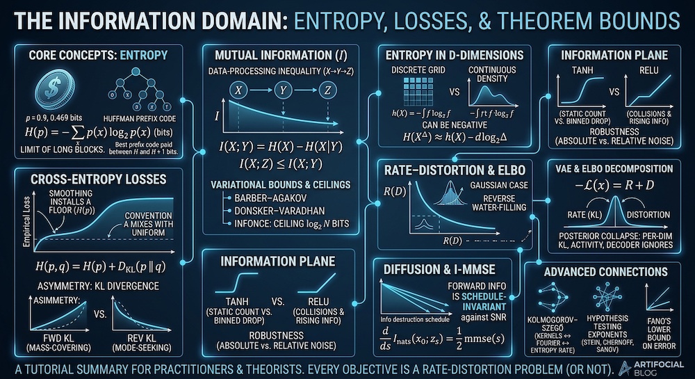
Start with the one sentence everything else hangs on, stated with the asymptote that is usually dropped. The entropy of a memoryless source is the number of bits per symbol you need to describe its draws, if you code optimally, in the limit of long blocks. For a single draw the best prefix code pays between and bits, and the gap closes only when every probability is a power of two. When the symbols are dependent the quantity that owns the compression limit is the entropy rate, , not the entropy of one symbol: draw one fair bit and set for every , and each symbol has bit while the whole sequence has one bit of uncertainty, so . §0 works with the memoryless case; §8 is about the processes where the two differ. Every result in this piece is a consequence of taking that sentence seriously — including the cases where a quantity that looks like an entropy is not one, and where a number that looks like a measurement is a property of the ruler.
Here is the claim, at the width the mathematics supports, because the tidy version is wrong in both directions. We are not claiming that machine learning is information theory wearing a hat, and we are not claiming that every budget you allocate is secretly a rate–distortion problem — §5 and Appendix D say exactly where that fails. The claim is this:
Information theory supplies a common language for several objectives you already optimise, but its connections operate at different levels. Cross-entropy and KL are related by an exact identity. Variational objectives split exactly into a distortion and an upper bound on rate — a decomposition of rate–distortion shape, whose rate meets Shannon's only where the family contains the optimum, as the linear-Gaussian example of §6 does. A stationary Gaussian process has an entropy rate determined by its power spectrum. Other connections — where a diffusion model's compute goes, what a fixed-size state can carry — are hypotheses whose consequences have to be established separately. The value of the lens is not that everything is secretly information theory. It is that it tells you which constraints are theorems, which quantities are measurements, and which analogies are bets.
Every connection in this piece carries one of four labels. If you are here for the floor under your loss, skip straight to §1 and come back to this table the first time a label stops you:
| Level | What it means | What you may conclude |
|---|---|---|
| L1 — exact theorem | The quantities and assumptions match a proven result | An identity or a bound you cannot beat |
| L2 — variational correspondence | The objective has the same optimisation structure, with every term defined | A formal analogy you can compute with |
| L3 — engineering heuristic | A similar resource–quality trade-off appears | Design intuition, to be validated |
| L4 — speculative analogy | A resemblance without a derivation | A hypothesis to test, nothing more |
Three running examples carry the same numbers through the whole piece, so that when two sections seem to disagree you can see which one is wrong. A -class classifier trained with label smoothing ( and , ): its floor in §1, its temperature in §1.1, its softmax as a variational identity in §9.8. A one-dimensional linear-Gaussian VAE (, , encoder ): its exact posterior, its ELBO level set and its rate–distortion frontier in §6, every number in closed form. An AR(1) process with unit innovation variance: the source of §5's real quantiser at , both spectral functionals in §8, and the length-scale callback in §11.3.
Prerequisites. Probability at the level of expectations and conditional distributions; logarithms; one linear-algebra fact (a log-determinant is a sum of log-eigenvalues); gradient descent. No prior information theory.
Two reading paths, and two sections neither may skip. The practitioner path is §0 → §1 → §2 → §3 → §5 → §6 → §7 → §12, doing the five checkpoint exercises that lie on it: exercise 1 closes §1, exercises 2 and 3 close §2.1 and §2.2, exercise 4 closes §6 and exercise 5 closes §7. The theorist path is §0 → §1 → §2 → §3 → §5 → §6 → §8 → §9 → §10 → §11, and adds the sixth exercise, which closes §8. §1 and §3 are on both paths: §1 holds the empirical-versus-population distinction and the one table that stops a floor being mis-subtracted, §3 is what §6 and §7 are built on, and §5–§6 are on the theorist's because they are the thesis. §4 (the information plane) is the one advanced branch neither path requires; take it by interest, and take §8 by interest if you are on the practitioner path. The history is Appendix A, the cross-field audit Appendix B, two toy models of ours Appendix C, and the graded ledger of how this piece bears on our earlier posts is Appendix D. This piece stands alone: where an earlier post of ours is relevant it is linked as a citation, the way a paper would be, and nothing below requires having read it.
Companion notebooks.
00_information_theory_from_scratch.ipynbbuilds entropy, cross-entropy, KL, mutual information, the information plane and a rate–distortion curve in pure NumPy;01_entropy_across_the_series.ipynbcarries the longer experiments — the entropy-rate identity, where a diffusion model's forward information goes and the I-MMSE check, the ELBO level set on the rate–distortion frontier, a real quantiser against its bound, a verification-noise toy, and what recursive training does to tails. Both ship fully executed, and every number in a code block below is copied from their printed output; the few remaining worked-example numbers come fromworked_numbers.py(27 numbered sections), with the arithmetic shown inline. Training is float64 throughout, and the float32 and float16 numbers of §4.2 are readout casts of the same activations, not networks trained at lower precision. Environment, seeds and the reproducibility scope — every printed number within the environment; the closed-form checks across platforms; the trained-network collision counts not — are printed by each notebook's first cell and discussed where they matter, in §4.2.
Units, once. We write and say bits unless a formula says otherwise; several results below are native to nats because the literature states them with , and mixing the two inside one bound is the most common way to get a wrong number out of a right theorem. The ledger:
| Quantity | Unit in this piece | Conversion |
|---|---|---|
| Shannon entropy , cross-entropy, KL, mutual information | bits () | for nats |
| Differential entropy , entropy rate (§3, §8) | nats where the formula has , bits where it has — stated at each table | for bits |
| Cross-entropy loss as a framework computes it | nats per token (mean reduction) | the floor tables give both |
| ELBO, rate , distortion (§6) | bits in the tables | for nats |
| Barber–Agakov (§3.1) | nats on both sides — the entropy of is converted before it enters the bound | first |
| Donsker–Varadhan, InfoNCE, MINE (§3.1, §10.1) | nats, as implemented: in the bound, ceiling | for bits; ceiling |
| I-MMSE and the diffusion loss floor (§7) | nats | for bits |
| Xu–Raginsky generalisation bound (§10.2) | in nats inside the square root | with in bits, multiply it by first |
0. One quantity, four costumes
Start with the definition and then immediately do something useful with it. For a discrete distribution over outcomes :
The standard gloss is "average surprise," which is true and slightly useless. The operational reading is better, and it has to be stated with its asymptote attached, because it is almost always stated without one:
is the number of bits per symbol you need to describe independent draws from , if you code optimally, in the limit of long blocks. For a single draw the number of yes/no questions is an integer, and the best you can do is bounded by — Shannon's bound for prefix codes, which Huffman's construction attains. The coin has entropy 0.469 bits and still costs one whole question per draw; block a hundred draws together and the cost per draw approaches 0.469. Entropy is the per-symbol cost of describing the source, which is Shannon's source-coding theorem (§9.1 sketches the proof), not the cost of describing one symbol — and for a source with memory that per-symbol cost is the entropy rate of the introduction, never more than of a single symbol and usually less.
Three sanity checks from the notebook, worth running once by hand so the numbers stop being abstract:
H(uniform over 8) = 3.000000 bits (exact: log2(8) = 3)
H(point mass) = 0.000000 bits (exact: 0)
H(dyadic skewed) = 1.875000 bits (exact: 1.875)Worked example — the one case where a single-symbol code is exact. The third distribution is padded to eight slots with three zeros. It is called dyadic because every probability is a power of , so the ideal code length is a whole number of bits for every symbol: . Assign the codewords 0, 10, 110, 1110, 1111 — a prefix code, so no codeword begins another and the stream decodes without separators. The expected length is
which equals exactly. A dyadic distribution is precisely when the prefix-code gap closes; every non-dyadic distribution pays a strictly positive penalty per symbol for rounding fractional bits up to whole codewords, and that penalty is what block coding and arithmetic coding (§9.2) remove. And the claim that uniform is the maximum has a two-line proof rather than a vote: by Jensen's inequality, since is concave. The expectation of counts the outcomes with positive probability, which is why the dyadic example padded with three zeros is bounded by and not only by ; equality throughout needs constant on a support of size , i.e. uniform. (The notebook's 200,000 random distributions on eight outcomes, none above 3 bits, are a picture of the inequality, not the argument for it.)
The single most useful intuition pump is the biased coin:
A fair coin is exactly 1 bit. A coin with is 0.4690 bits — nine-to-one odds have already destroyed more than half the uncertainty of a fair coin.
Remember that shape. Entropy falls off fast as a distribution concentrates, which is why a model that is "only somewhat confident" has already given away most of its uncertainty, and why calibration errors in the confident regime cost more than they look like they should.
The four costumes
Everything below is built from and two relatives:
- Cross-entropy — the cost of coding 's data with 's codebook.
- KL divergence — the excess cost of that mistake.
- Mutual information — how much learning shrinks your uncertainty about .
And the identity that makes the first two the same object:
We verified it over 20,000 random pairs — maximum absolute deviation 8.882e-16, which is floating-point noise. Be clear about what such a check is: it validates that our implementation agrees with an algebraic identity, and nothing else. It is not evidence for the identity (the proof is one line: expand the log of a ratio) and it does not vouch for any other experiment in the notebooks. We say this once here so that no later "agrees to " is read as more than the software test it is.
What the identity buys you is the most under-appreciated line in applied machine learning:
Minimising cross-entropy against a fixed target is exactly minimising KL divergence to that target, because does not depend on your parameters. Minimising the population cross-entropy is a KL projection of the data distribution onto your model class. Training minimises the cross-entropy of the empirical distribution — a KL projection of the training sample — and the two coincide only in the large-sample limit, under conditions that are usually left unstated (a fixed model class, independent draws, a minimiser that exists and is found). We say "empirical" once here and mean it wherever a training loss appears below.
It does not follow that every classifier is doing variational inference. That claim needs a latent variable and an approximate posterior, and it is made — correctly, with its assumptions — in §6.
1. Your loss has a floor, and you built it yourself
Here is the first place the theory pays rent. Practitioners routinely watch a training loss plateau above zero and reach for the usual explanations — underfitting, a bad learning rate, insufficient capacity. Often the correct explanation is arithmetic: you added label smoothing, and label smoothing installs a floor.
If your targets are smoothed, the target distribution is no longer a point mass, so . By the identity in §0 the best achievable cross-entropy is not zero — it is , reached when exactly. But "smoothed" is not one distribution, and a floor table that does not say which one it used is useless. There are two conventions in common use:
- Convention A — mix with uniform over all classes: , so the true class gets and every other class gets . This is what
label_smoothing=does in PyTorch'sCrossEntropyLossand in most frameworks that copied it (Szegedy et al., 2016). - Convention B — hold the true class at and spread over the other classes, each. The companion notebook prints both conventions; the table below is its convention-B table, and the convention-A row worked by hand after it is reproduced by the notebook to the same digits.
The notebook's table, convention B:
Irreducible cross-entropy floor H(p) induced by label smoothing
K eps floor [bits] floor [nats]
10 0.00 0.000000 0.000000
10 0.10 0.785988 0.544805
1000 0.10 1.465430 1.015758
128000 0.00 0.000000 0.000000
128000 0.05 1.134686 0.786504
128000 0.10 2.165573 1.501061
128000 0.20 4.115083 2.852358Worked example — the same row under convention A, by hand. , : the true class gets and each of the other nine gets .
with four-decimal intermediates — the hand line is the rounded one. Unrounded it is 0.721763 bits (0.500288 nats), which is the notebook's convention-A row and the checkpoint value at the end of this section.
So the two conventions give 0.722 bits (0.500 nats) and 0.786 bits (0.545 nats) for the same nominal at — a 9% difference in the floor, large enough to misdiagnose a run. At the difference vanishes: convention A gives 2.165557 bits / 1.501050 nats against B's 2.165573 / 1.501061, because on the true class is negligible when is six figures. The large-vocabulary warning therefore survives either way:
A vocabulary of 128,000 tokens with cannot go below 1.501 nats under either convention. A model sitting at 1.52 nats is not underfitting; it is within 0.02 nats of the per-example floor of its own smoothed objective on clean labels, and it will be reported as broken by anyone comparing against a run that used . The same costs about 0.5 nats at and 1.5 nats at — the floor scales with vocabulary, which catches people moving between model families.
Procedure 1 — read the floor off the tensor. (i) Materialise one target row exactly as it reaches the loss: after smoothing, after any mixing or masking. (ii) Compute in the log base your loss uses. (iii) Apply the same reduction your loss applies (
meanover which tokens,sum, non-padding only). (iv) That number — not a table, not the convention you believe your framework uses — is your floor on clean labels. On noisy labels there are two more floors, and rule 3's table says which loss each belongs to.
Practical rules, in order:
-
Read off the tensor you actually pass to the loss — Procedure 1 above. It is a one-line check and the only one that cannot be wrong about the convention.
-
Check the reduction.
meanover tokens gives a per-token floor in the units above;sumscales it by the token count; a loss averaged over non-padding tokens only has yet another denominator. The floor must be computed in the same units as the loss you are reading. -
Training loss and held-out loss have different floors, and there are two held-out losses. On training data with hard labels the floor is zero and a memorising model can reach it. On held-out data the labels are uncertain — is not a point mass — and which floor applies depends on which loss you score. Under convention A the expected smoothed target at is , and the four cases at one point, , , , are these (
worked_numbers.py§11):the target you score against minimiser floor at that point what it is smoothed — the loss you trained bits the held-out floor of the smoothed objective hard label — what most validation code computes bits the held-out floor of the hard-label objective hard label, but scored at the smoothed optimum — bits attains neither floor " plus the table's " — bits wrong — the two entropies do not add The additive formula errs in the dangerous direction: a floor is a minimum, so overstating it makes a model at 0.6 bits look as if it had beaten its floor, and that is the misdiagnosis. The fair-label counter-example ( independent of ) hides the first three rows, because then for every and every floor is exactly 1 bit — while the additive formula says 1.286. Subtract 0.584 from a hard-label curve and you have subtracted the wrong floor. Both noisy-label floors need , so neither is readable from the targets alone; §9.4 (Fano) is the tool for bounding .
The restriction, and what is not. Convention A is the target you would get from uniform label noise at rate , but is a regulariser you chose, not an estimate of a noise rate: a model on its smoothed floor is optimal for the objective you wrote down, is not evidence that the labels are noisy at rate , and by construction reports 0.86 where — miscalibrated relative to the truth while sitting exactly on its floor. Excess over the floor is a statement about the objective you trained; calibration is a separate measurement, and §1.1 says how to make it.
-
Compare excess loss, never raw loss, across runs that differ in smoothing, vocabulary or tokenizer. And across tokenizers, per-token loss is not comparable at all: a tokenizer that produces more tokens per byte spreads the same information over more loss terms. Report bits per byte (total log-loss over the byte count of the text) when the vocabularies differ; it is the one unit that survives the change.
-
Distillation has the same floor. Training a student by cross-entropy against a teacher's soft distribution is KL to a target with its own entropy; the student's loss cannot go below the teacher's mean per-token entropy, and a student that reaches it has matched the teacher, not failed to beat it.
-
Every floor, and every number in this piece, assumes a distribution. On shifted data the identity in §0 reads : a model that sat at its floor on the training distribution pays the full KL to the new one, and the floor itself moves, because is a property of the distribution rather than of the task's name. A perplexity measured on text from a different source than the training set is a codelength under the wrong code; a mutual-information estimate (§2.2) or a Fano floor (§9.4) computed under one distribution says nothing under another. Say which distribution every information quantity was computed under, and re-measure after a shift rather than carrying the number across.
1.1 Perplexity, temperature, and what a proper scoring rule does and does not promise
Perplexity is when is in bits, in nats — the effective number of equally likely options. For a language model the quantity reported is the exponential of the held-out cross-entropy per token, , which is the model's codelength on text it did not see. It is not the entropy of the model's own next-token distribution; those agree only when the model is the true distribution. A perplexity of 17 means the model's held-out surprise matches a uniform choice among 17 tokens.
Temperature is a direct entropy dial on that next-token distribution. From the notebook, for a single distribution over with logits drawn from :
T H [bits] perplexity p(top-1) 90% mass in
0.1 0.1817 1.13 0.9725 1 tokens
0.3 1.1949 2.29 0.7264 2 tokens
0.7 3.3020 9.86 0.3431 11 tokens
1.0 4.0870 16.99 0.2176 17 tokens
1.5 4.7595 27.09 0.1289 25 tokens
2.0 5.0904 34.07 0.0914 33 tokens
100.0 5.6436 49.99 0.0208 45 tokensTwo things are worth extracting. First, the "90% mass in" column is the one that predicts sampling behaviour, and it is wildly nonlinear in : going from to takes the nucleus from 2 tokens to 11. That is the range where most production sampling lives, and it is where small temperature changes have the largest effect on what can come out. Second, the limit: uniform over is bits, and at we measured 5.6436 — the logits have been thrown away. High temperature does not make a model creative; past a point it makes the model absent.
Now the point about scoring rules, which this table is the right place for. Cross-entropy is a strictly proper scoring rule: its expectation under the true distribution is uniquely minimised by reporting the true distribution. That is why it is the right training loss for probabilities. It is not a promise that a low loss means a calibrated model, and the table shows why in one column: every row has the same , so every row has the same accuracy, while the loss and the calibration change with . Temperature scaling (Guo et al., 2017) fits exactly this one parameter on held-out data to minimise cross-entropy, and it typically fixes the calibration of an over-confident network without touching a single prediction. So: a loss gap between two models can be a calibration gap rather than an accuracy gap, and the way to tell is to measure accuracy and a reliability diagram separately rather than to read either off the loss. (The Brier score is the other proper scoring rule you will meet. It is bounded, which makes it gentler on confident mistakes and less informative about them; choosing between the two is choosing how to price confidence, not choosing which one is correct.)
1.2 KL is not a distance, and the asymmetry is a design decision
, and the gap is not a technicality — it determines what your model does when it cannot fit the target. Measured:
p = uniform(4), q = nearly a point mass
KL(p||q) = 5.475422 bits (mass-covering: punishes q for ignoring p's support)
KL(q||p) = 1.965781 bits (mode-seeking: q only has to sit somewhere p allows)
ratio = 2.79x — 'KL distance' is not a distance.Forward KL is mass-covering. It integrates against , so wherever the data has mass and your model does not, you pay. Under a model family too simple to fit every mode, the minimiser spreads itself across the modes. This is maximum likelihood. Reverse KL is mode-seeking. It integrates against , so the model is only penalised where it puts mass, and it can ignore an entire mode for free. This is the variational objective, and it is the standard explanation for why mean-field variational inference under-estimates posterior variance.
Hold the generative-modelling corollary loosely. "Forward KL makes blurry images, reverse KL makes sharp ones" is a tendency under a misspecified unimodal family, not a law. Whether a maximum-likelihood model's samples look blurry depends on the likelihood you chose — a per-pixel Gaussian likelihood is what produces averaged images, and a model with the same KL direction but an autoregressive or flow likelihood does not — on whether the family can reach the modes at all, and on how you sample at generation time. The asymmetry tells you which mistakes the objective forgives. It does not tell you what the pictures look like.
The degenerate case matters more than the ratio:
p with a zero where q is positive: KL(p||q) = 1.000000 bits (finite)
the same pair the other way round: KL(q||p) = infAn infinite KL is not a numerical problem to be clipped away — it is the objective telling you that places mass where says the event is impossible. If you are clamping KL terms to keep training stable, you are suppressing a signal about support mismatch. Look at the support first. (When supports genuinely differ by design — two disjoint datasets, two generators — KL is the wrong instrument altogether; Jensen–Shannon, total variation or a Wasserstein distance are the ones that stay finite, and §10.4 needs total variation for exactly this reason.)
1.3 The numerical box: how to actually compute it
One concrete engineering section, because cross-entropy's failure modes are silent and its cost profile surprises people.
Take logits, not probabilities. The cross-entropy of a softmax is , and the second term must be computed as a shifted log-sum-exp, with . The notebook shows what happens otherwise:
naive softmax vs shifted softmax
dtype=float64 max logit 100: naive finite? True naive[0]=0.66524095 shifted[0]=0.665241
dtype=float64 max logit 800: naive finite? False naive[0]=nan shifted[0]=0.665241
dtype=float32 max logit 100: naive finite? False naive[0]=nan shifted[0]=0.665241
float32 overflows at exp(~88). Models train in float32 or bfloat16. Shift, always.A logit of 100 is not exotic in a large model, and in bfloat16 the usable range is the same as float32 with far fewer mantissa bits. Keep the logit tensor in at least float32 for the loss even when the rest of the model is in half precision; a cross-entropy kernel that accepts probabilities has already lost the game before it starts.
Mask zeros, do not clip them. The term at is and must be defined as zero. The tempting alternative — clipping probabilities to — does not error, does not warn, and changes the answer by an amount that depends on and on how many zeros the distribution has:
masked H(p) = 0.8812908992 bits (correct)
clipped H(p) at eps=0.001 = 0.9127844694 bits error +3.15e-02
clipped H(p) at eps=1e-06 = 0.8813523780 bits error +6.15e-05The loss layer can be the most expensive thing you run. The logit tensor is , and vocabulary is now six figures. Cut Your Losses in Large-Vocabulary Language Models (arXiv:2411.09009) reports that for small models the cross-entropy layer consumes an order of magnitude more memory than the rest of the model combined, and reduces the loss computation's footprint from 24 GB to 1 MB on Gemma 2 (2B) by never materialising the full logit matrix. The last conceptual step of your model is often the most expensive thing in the training loop. That is worth knowing before you buy more accelerators.
Checkpoint exercise 1 (floors). Materialise one row of your own training targets under your framework's label smoothing and compute its entropy in the units of your loss. Then prove that under convention B the floor is exactly , check it against the and rows, and show that under either convention it grows as plus a constant. Finally, for a fair label independent of the input, show that the held-out floor under convention A is 1 bit at every . Checkpoints: , : 0.785988 bits (B), 0.721763 bits (A); the independent-label floor is , not .
2. Mutual information, and the law that says post-processing cannot help
Mutual information is the natural measure of "how much does knowing this tell me about that," and its most useful form is the third one below:
Mutual information is the KL divergence between the joint and the product of the marginals — a measurement of how far from independent two variables are, in the same units as everything else. For the binary symmetric channel — uniform, equal to flipped with probability — the closed form is , with the binary entropy. Measured against it:
f I(X;Y) measured 1 - H(f) exact
0.00 1.000000 1.000000
0.01 0.919207 0.919207
0.10 0.531004 0.531004
0.25 0.188722 0.188722
0.50 0.000000 0.000000Note the shape: a 10% error rate costs you nearly half the bit. Channel capacity degrades much faster than error rate suggests, which is the same lesson the biased coin taught in §0, and which is why "97% accurate" and "99% accurate" are not a 2% difference in information terms.
2.1 The data-processing inequality, with its proof
If is a Markov chain — depends on only through — then
Proof sketch (three lines). Expand by the chain rule in both orders: . The Markov property says — given , tells you nothing further about . Conditional mutual information is non-negative (it is a KL divergence), so , and therefore . Equality holds exactly when , i.e. when is a sufficient statistic of for — the processing threw away only what was irrelevant.
Worked example — a cascade of two noisy stages, by hand. Let be a fair bit, let be passed through a binary symmetric channel with flip probability , and let be passed through a second identical channel. The first stage leaves bits (the table above). Two independent flips compose into one flip with probability , so . Now , giving bits. The second stage destroyed bits, and no decoder placed after — however large, however well trained — sees more than 0.320 bits about . That is the whole inequality in one pipeline.
(The notebook also runs the inequality on 5,000 random Markov chains and finds no violation — a software test of our implementation, not evidence for the theorem.)
What the DPI does and does not say about your pipeline. It says your preprocessing is a hard ceiling on the information available to the Bayes-optimal predictor downstream: a frozen encoder bounds every head you attach, an early quantisation step bounds every later architecture, and nothing recovers what was removed. It does not say that a step which loses information will hurt a model you can actually train, and it says nothing at all about steps that lose none — keep the two kinds of preprocessing apart. Standardising a feature, with fixed and , is invertible, so exactly: mutual information is invariant under invertible maps of either variable, and whatever standardisation does for optimisation it does without moving the ceiling. Cropping, quantising and discarding nuisance variation are non-invertible; they lower the ceiling, and a finite-sample learner — which is not the Bayes-optimal predictor — routinely gains held-out accuracy from them anyway, because they shrink the hypothesis space it has to search with the data it has. That is the practitioner's version of the inequality: an operation can make information easier for a finite model to use without changing, or while reducing, what an ideal predictor could extract. So when a bigger model fails to beat a smaller one on the same features, the DPI is one hypothesis — the information is not in the features — and it is a hypothesis you can test rather than assume: estimate how much information is there (§2.2, carefully) and turn it into a floor on error with Fano's inequality (§9.4). Learnability and information are different ceilings, and only the second one is what this theorem bounds.
Checkpoint exercise 2 (data processing). Three BSC() stages in series: derive the composite flip probability and compute for . Then exhibit a Markov chain with and , and say what that makes . Checkpoints: composite flip ; bits, below the two-stage 0.320; equality needs to be a sufficient statistic of for .
2.2 Your mutual-information estimate is a measurement with an error bar you have to earn
Here is the part that should change how you read papers. The formulas above take a distribution as input. In practice you have samples, and the obvious move is to build a histogram and put it through the formula. That plug-in estimator has a known leading-order bias: on a fixed table with every cell probability positive, in the large- regime,
(the Miller–Madow correction applied to the three entropies in ). The notebook measures this against a ground truth of exactly zero — and drawn independently on an table:
TRUE mutual information is 0.000000 bits (X and Y drawn independently, 8x8 table)
N mean I_hat std predicted bias ratio
20 1.388577 0.193090 1.767301 0.786
50 0.803480 0.108236 0.706921 1.137
200 0.196598 0.038791 0.176730 1.112
1000 0.035860 0.007079 0.035346 1.015
5000 0.007059 0.001517 0.007069 0.999
100000 0.000347 0.000068 0.000353 0.981At on an table, the estimator confidently reports 0.197 bits between two independent variables. For scale, a perfectly informative binary variable carries 1.000 bits. The correction formula tracks well in the regime it was derived for and fails where you would most want it: at it predicts 1.767 bits while the estimator reports 1.389. The asymptotic expansion is unreliable when the table has fewer samples than cells, which is the regime it exists to describe. The correction is a diagnostic, not a rescue. And the bias does not cancel when there is a real signal:
N true I I_hat error
50 0.53100 0.54576 +0.01476
200 0.53100 0.53917 +0.00817
1000 0.53100 0.53184 +0.00084
10000 0.53100 0.53096 -0.00004Now a correction to a rule you will see stated often: treat every mutual-information estimate as an upper bound. That is not generally true. The leading-order term is positive, so under independence and in the large-sample regime the estimate is an over-estimate. But the bias of the plug-in estimator is not positive for every distribution and sample size, and a one-line counter-example settles it: let be a fair bit, so bit exactly, and draw one sample. The empirical joint is a single cell, , and — an under-estimate by a full bit. More generally, a strongly dependent pair observed on a sparse table under-counts its own dependence, while an independent pair on a sparse table over-counts. The sign of the error depends on the distribution, the table and , and no single correction knows which case you are in.
Procedure 2 — how to report a mutual-information estimate. Treat it as an uncertain, estimator-dependent measurement, not as a bound in either direction, and report four things with the number. (i) and the estimator — bins and their count, or the nearest-neighbour , or the critic and batch size. (ii) A permutation null: shuffle , re-estimate, repeat a thousand times — that is the distribution of under independence at your and your bins, the only null that matters — and report its 95th percentile beside your estimate. (iii) A bootstrap interval for the spread. (iv) For a difference between two setups, in this order. First name the estimand both numbers estimate — the same quantity, on the same variables, under the same discretisation — because two plug-in values at different or different bins are estimates of different things until you have said why they are not: the bias term above moves with both, and so does the regime in which it is valid. Raw numbers across unmatched settings are not a comparison; they become one only once the bias of each estimate has been accounted for and the uncertainty of each carried through, which is possible and is work. Second, if the settings are matched, the comparison is controlled, not corrected: matching removes the sample-size and binning contributions and leaves the part of the bias that depends on the underlying distribution, so two matched estimates can still carry different biases. Matching is a useful experimental control — neither a requirement nor a sufficient correction. Third, keep the test and the interval apart. The permutation null of (ii) tests one stated null, independence under exchangeability, and that is all it tests; it is not an interval for a difference. The interval comes from a resampling procedure built for the difference — paired when the two estimates share observations, independent-sample otherwise. If a paper reports that layer 5 carries more information than layer 3, this is the list to check before believing it.
Histograms are not the only estimator, and in more than a few dimensions they are the wrong one. Nearest-neighbour estimators (Kraskov, Stögbauer & Grassberger, 2004) avoid binning and have their own small-sample failure modes; neural estimators such as MINE (arXiv:1801.04062) exist because both fail in high dimensions, and they carry variance pathologies of their own. §3 states the variational bounds that make the neural ones principled, and the ceiling that caps the most popular of them. There is no free estimator.
Checkpoint exercise 3 (estimation). Reproduce the independence experiment at with a 1,000-shuffle permutation null, and report the 95th percentile of under the null. Then construct a dependent distribution and a sample size at which the plug-in estimate is biased downward, and state why. Checkpoints: the notebook's null has its 95th percentile at 0.265 bits, with the single observed estimate at 0.229 inside it; at gives against a truth of 1 bit.
3. Discrete and differential entropy are different objects, and you need both before the next five sections
Everything so far was discrete. The next five sections involve Gaussian noise, continuous latents, diffusion processes and kernels, and every one of them is a trap if you carry the discrete intuition across unchanged. Here is the boundary.
For a density on the differential entropy is , and it is not a count of anything:
- It can be negative. A uniform distribution on has bit. A Gaussian with variance has , which is 2.047 bits at and negative once .
- It is not a file size. A continuous value has infinitely many bits; there is no lossless code for it.
- It is invariant under translation and not under scaling: for a scalar acting on , , and for an invertible matrix , . Rescale your features and your "entropy" moves by a constant that grows with the dimension.
What does connect it to bits is quantisation, and the correction carries the dimension. Discretise on a cubic grid of side and the entropy of the discrete variable obeys
each cell has volume , not , so the correction is one per dimension.
Worked example (worked_numbers.py §5 and §15). A unit Gaussian in one dimension at : bits, and the binned entropy computed exactly is 5.3696. In two dimensions, with independent standard coordinates, bits and the grid entropy at is bits (exact: 10.7392); the one-dimensional formula would say 7.416 and be wrong by a full . Halve and you add one bit per dimension, forever; the differential entropy is the part that does not depend on your ruler. §6's remark that a continuous reconstruction term becomes a codelength only after fixing a precision is this formula with equal to the data dimension.
That last sentence is why mutual information survives the passage to continuous variables and entropy does not. Write and the terms cancel: each variable's own dimension and bin width appears once with each sign. So is well-defined, finite under mild conditions, and invariant under smooth invertible transformations of either variable — which is why it is the right currency for representations (§4) and channels (§7), and why differential entropy on its own almost never is.
Two consequences you need before going on:
- A deterministic continuous map has infinite mutual information with its input. If with continuous and smooth and non-degenerate, then and . If instead takes finitely many values, is finite and bounded by the input's entropy. These are two different probability models and they give different answers; §4 shows what goes wrong when you quote the first in an experiment built on the second.
- The Gaussian is the maximum-entropy density at a given variance (and at a given covariance in dimensions), so for a channel with Gaussian noise of variance and a Gaussian input of variance , bits per use. In isotropic dimensions, multiply by . That formula is what §7's diagnostic evaluates for a Gaussian source; the relation that owns the floor there is I-MMSE, for any finite-power input, and §7 displays it with its factor of one half in the same line as the number it produces.
3.1 The variational bounds, and the ceiling on the most popular one
Estimating in high dimensions means bounding it with something you can train. Three bounds carry most of modern representation learning, and they are worth stating because each says exactly what its estimate means.
All three are stated in nats, because that is how every implementation computes them: the critic's cross-entropy is a natural log, and the bound has to be read in the same unit.
Barber–Agakov (2003). For any conditional model ,
with both terms in nats: the entropy of has to be converted from §0's bits before it enters (), and a bits-valued added to a nats-valued log-likelihood is not a bound on anything. For continuous replace by the differential entropy and read as a density; under the usual finiteness conditions the bound is still exact, and it is tight when equals the true conditional almost everywhere. Check on the BSC(0.1) of §2 with a uniform bit and the true conditional (worked_numbers.py §19): , , sum nats bits, which is exactly; with left in bits the sum would be , a number with no meaning. A decoder that predicts from gives a lower bound; a better decoder gives a tighter one; the bound needs the entropy of , which you have when is something you constructed and have to estimate otherwise.
Donsker–Varadhan. over all functions ; divide the whole expression by for bits. Restrict to a neural network and you have MINE. Be careful about what is a bound: the population quantity, for any fixed , is a lower bound on ; the number a finite-sample, optimised MINE run prints is not, because the supremum is taken over the same sample it is evaluated on and can overshoot the true — and its variance grows exponentially with the true , which is the pathology §2.2 mentioned.
InfoNCE (van den Oord, Li & Vinyals, 2018). Draw one positive pair and negatives, train a critic to pick the positive, and with the critic's cross-entropy in nats, . The two terms must be in the same unit — a ceiling subtracted from a nat-valued loss is the mistake to avoid. This is the objective under contrastive representation learning, and its ceiling is the thing to remember: the bound can never exceed nats, i.e. bits (Poole et al., 2019). With candidates per positive — one positive and 4,095 negatives — the estimate saturates at nats bits regardless of how much information the representation actually carries (a batch of 4,096 negatives has ; the count that enters the ceiling is the total). A contrastive loss that has stopped improving may have hit the batch, not the data.
The pattern across all three is the same one as §2.2: an estimate of mutual information comes with the estimator's name attached, and the estimator's ceiling or its variance is part of the number.
4. The information plane, and the most contested measurement in the field
Saxe et al. (ICLR 2018) showed that the compression phase of the information plane is a property of double-sided saturating nonlinearities read through a binned estimator, not of stochastic gradient descent: it appears with tanh, it does not appear with ReLU or with linear units, and where it appears it has no evident causal link to generalisation. That is the sentence this section starts from, and everything below is an addition to it rather than a rediscovery of it. The claim it answers is the information bottleneck (Tishby, Pereira & Bialek, 1999; Tishby & Zaslavsky, 2015), which proposes that a good representation of input for predicting solves
keeping what predicts and discarding everything else, together with the famous empirical claim (Shwartz-Ziv & Tishby, 2017) that training has two phases — a short fitting phase where rises, then a long compression phase where falls while accuracy holds. Goldfeld et al. (2019) supplied the other half of the objection: once noise makes finite and estimable, what the estimate tracks is geometric clustering of the representations. Neither is in dispute here. What our experiment adds is not a fourth estimator but two things an estimator cannot give: an input with finite support and exactly known entropy, so that is a quantity you count rather than estimate, at every checkpoint; and a noisy readout whose information is an integral over a known mixture, with a standard error, no bins, and both absolute and scale-normalised noise. The first is a lemma about the quantiser. The second is the measurement that generalises, and it comes first.
We built the task — all 4,096 twelve-bit patterns, uniform, so bits exactly — trained a tanh network and a ReLU network (hidden widths 10, 7, 5, 4, 3) to convergence, and measured. Both learned the task:
tanh: final epoch 4000 loss 0.00008 nats train accuracy 1.0000
relu: final epoch 4000 loss 0.03921 nats train accuracy 0.98904.1 The measurement that generalises: a noisy readout, at two scales
A deterministic layer read at the precision it was computed in — float64 here, NumPy's default — is one readout channel among several, and not the one most consumers of the layer have: a deterministic forward pass at that precision does read it that way, while a lower-precision serving path, a sensor, or the next layer's own tolerance read through something coarser — and whether a given precision actually merges any of the 4,096 inputs depends on the activation values and the format, which is why §4.2 recounts the same weights after a cast to float32 and to float16, and why the measurement below varies the channel explicitly rather than assuming one. So the question with operational content is how much of the input's identity survives a readout through a stated noise channel: with added to the activations. Because is uniform over a known set of 4,096 points, the density of is a 4,096-component Gaussian mixture with known components, and is an ordinary Monte Carlo expectation of — no learned estimator, no bins, none of the ceiling of §3.1, and an error bar. (The printed label's "exact" refers to the density being known exactly; the integral is Monte Carlo, and the standard error shown is the one that matches the design: every input is present by construction with four independent noise draws each, so the variance of the estimate is the sum of the per-input variances over — a stratified error bar — not the pooled spread of all the values, which also counts the between-input spread of the conditional means and is conservative. The notebook prints both and a 16-draw rerun of two cells, and the 4-draw bars hold.) The column headed H(T) exact is the limit, and §4.2 says why it is a count rather than an estimate. First the table with the same absolute on both networks:
Stochastic representation: I(X; T + N) in bits, N ~ N(0, sigma^2 I) on the activations,
computed as an exact Monte Carlo expectation over the known 4,096-component mixtureThree things to read off it. First, at — a hundredth of the activations' RMS — tanh layer 3 carries 4.2 bits rather than its float-precision 12, and layer 5 carries 1.6: whatever the deterministic layer holds, a whisper of noise removes most of it, which is what "tightly clustered" means in bits. Second, this is Goldfeld et al.'s mechanism on our own numbers: once noise makes the quantity finite, what it measures is how far apart the activation vectors sit relative to , and the tanh network's deep layers cluster far more tightly than the ReLU network's. Third, the ordering of the two networks flips between the exact and the noisy columns: exactly, tanh carries more (12 against 7.22 bits at layer 5); at each of the three noise levels, ReLU carries more in every hidden layer but the first.
But the absolute table does not control for scale, and the flip depends on it. The noise has the same absolute standard deviation in both networks while the activation scales differ — RMS 0.978 at the deepest tanh layer against 3.881 at the deepest ReLU one — so is a four-times-smaller relative perturbation of the ReLU representation, and a downstream affine layer can absorb any rescaling of its inputs for free. The comparison that survives a change of scale is the same measurement on standardised activations, , with now a fraction of each layer's own RMS. One layer-wide RMS removes a global scalar and nothing more: for an invertible matrix , but in general , so both tables are statements about robustness under isotropic Gaussian noise in the coordinates the network produced, not a representation-invariant notion of intrinsic robustness:
Scale-normalised stochastic representation: I(X; T/RMS(T) + N) in bits, N ~ N(0, sigma^2 I),
so sigma is now a fraction of the layer's own RMS activation (same Monte Carlo integration, same seeds).
act layer act.RMS H(T) exact | rel sigma=0.01 | rel sigma=0.1 | rel sigma=0.5
tanh 1 0.719 12.0000 | 12.000 +/-0.000 | 11.242 +/-0.008 | 5.227 +/-0.016
tanh 2 0.847 12.0000 | 9.617 +/-0.009 | 4.943 +/-0.011 | 1.944 +/-0.009
tanh 3 0.947 12.0000 | 4.268 +/-0.008 | 2.117 +/-0.006 | 1.262 +/-0.005
tanh 4 0.897 12.0000 | 2.479 +/-0.006 | 1.433 +/-0.004 | 1.088 +/-0.003
tanh 5 0.978 12.0000 | 1.606 +/-0.004 | 1.199 +/-0.002 | 1.043 +/-0.002
relu 1 1.013 12.0000 | 11.868 +/-0.003 | 8.407 +/-0.013 | 3.003 +/-0.012
relu 2 1.847 12.0000 | 9.358 +/-0.009 | 4.696 +/-0.009 | 2.211 +/-0.008
relu 3 2.598 11.9609 | 7.664 +/-0.009 | 4.046 +/-0.008 | 1.835 +/-0.008
relu 4 3.396 11.9609 | 7.226 +/-0.008 | 3.951 +/-0.008 | 1.683 +/-0.008
relu 5 3.881 7.2237 | 4.580 +/-0.006 | 2.696 +/-0.006 | 1.270 +/-0.007Now the flip can be attributed. In the three deepest layers it survives normalisation, so it is shape and not scale: at a relative of 0.01 the ReLU network carries 7.66, 7.23 and 4.58 bits in layers 3, 4 and 5 against the tanh network's 4.27, 2.48 and 1.61 — and the ReLU figures fell when scale was removed (5.61 → 4.58 at layer 5, because its RMS of 3.881 had made the absolute a quarter-percent perturbation), while the tanh figures barely moved. The ReLU layers keep more information under matched relative noise because their activation vectors are spread more evenly relative to their own scale — the geometry the effective-rank column of §4.2 hints at for layers 3 and 4 (1.31 and 1.54 for ReLU against 1.05 and 1.03 for tanh), while at layer 5 both networks have an effective rank near 1 and the difference is how far apart the values sit along that one direction (2,271 distinct levels of a single live rectifier against 4,096 vectors packed into a cloud a hundredth of their RMS wide). In layer 2 the flip was scale: absolutely, ReLU led (10.25 against 9.34 bits at ); relatively, tanh leads at the two finer levels (9.62 against 9.36, and 4.94 against 4.70 at ), because layer 2's ReLU RMS of 1.847 against tanh's 0.847 had bought it a factor of two in relative noise — and at the coarsest relative level, 0.5, ReLU edges ahead again (2.21 against 1.94), so layer 2 is the one place where the ordering genuinely depends on the noise level. Layer 1 is tanh's under both. So the honest version of "ReLU is the more robust representation" is narrower than the absolute table suggested and still true where it matters: in the layers where the tanh network has collapsed onto one direction, ReLU carries more about the input through noise at any scale we measured; one layer up, the ordering is a scale artefact.
What the two tables separate is two questions that the single word "robust" runs together: which representation keeps more information at the scale the network produced (the absolute table), and which has the more information-preserving geometry once scale is factored out (the relative one). Where they disagree, the disagreement is scale, not shape. Both are measured under two controlled channels — absolute and RMS-normalised isotropic Gaussian noise — and the orderings are findings about those channels on these two networks, not an architectural ranking independent of readout noise or parametrisation. Three noise levels are three points, not a curve, and we claim neither ordering for any between or beyond them. The notebook draws all of it on one figure — the exact count, the binned value at three bin counts, and the noisy readout at three absolute and three relative levels, per layer and per network — so that the three rulers can be seen disagreeing on the same axes.
4.2 The lemma under it: on a finite input, , and you can count it
has finite support and is a deterministic function of , so by §3, bits. There is no infinity anywhere in this setup; the familiar claim that " is infinite for a deterministic network" is true for a continuous input and false for ours. And the exact value needs no estimator: count the distinct activation vectors over the 4,096 inputs and take the entropy of their empirical distribution. The notebook does this for every layer at the end of training, beside the 30-bin value, the effective rank of the layer's activation covariance (the exponential of the entropy of its normalised eigenvalues) and the fraction of units that are constant on the whole input set:
Exact I(X;T) = H(T) at float64 precision (the dtype the network was trained and read in), final epoch, vs the 30-bin value
act layer width distinct H(T) exact 30-bin eff.rank const units
tanh 1 10 4096 12.0000 11.9893 2.441 0%
tanh 2 7 4096 12.0000 8.4147 1.186 0%
tanh 3 5 4096 12.0000 3.6580 1.053 0%
tanh 4 4 4096 12.0000 2.0854 1.030 0%
tanh 5 3 4096 12.0000 1.5376 1.026 0%
relu 1 10 4096 12.0000 8.3856 1.717 0%
relu 2 7 4096 12.0000 5.6741 1.572 0%
relu 3 5 4065 11.9609 4.9885 1.313 40%
relu 4 4 4065 11.9609 5.1328 1.537 25%
relu 5 3 2271 7.2237 3.3971 1.000 67%Every tanh layer carries all 12 bits about the input at the end of training — at float64 precision, the dtype the notebook trains and reads in, which is the quantiser this sentence depends on, and §4.1 has already shown how little of it survives a coarser one. Read it as a statement about a readout channel: a downstream layer that reads these activations at the same float64 precision can in principle recover the input; what a float32 or a float16 consumer of the layer sees is a different map, and the next table counts it. Layer 3 — whose binned value fell from 11.85 to 3.66, the "8.19 bits of compression" of §4.3 — maps every input to its own activation vector. Its effective rank of 1.05 across five units says what actually happened: the activations collapsed onto essentially one direction, tightly clustered, so a 30-level quantiser merges most of them. The ReLU network is the one that genuinely loses information, and every loss is a collision — two inputs sent to the same activation vector: layer 5, with 67% dead units and a single live rectifier, maps the 4,096 inputs onto 2,271 vectors, bits, and layers 3 and 4 each merge a handful. Which of those collisions the dead units explain is a separate question, and the per-checkpoint table answers it.
The precision is part of the measurement, so the notebook varies it. Every array in the notebook is float64 — NumPy's default; nothing in it is float32 — so "distinct" above means distinct as float64. A consumer that reads the layer at lower precision reads a different map, and the exact count has to be redone for that map. The notebook casts the same float64 activations — same weights, same forward pass — to float32 and to float16 before counting. These are readout casts, not networks trained at lower precision, which would move the weights as well as the readout:
Readout-precision ablation: distinct activation vectors and H(T) [bits] when the float64 activations
are CAST to a narrower dtype before counting (same trained weights; the cast is at the readout only).
act layer | float64 | float32 cast | float16 cast
tanh 1 | 4096 12.0000 | 4096 12.0000 | 4096 12.0000
tanh 2 | 4096 12.0000 | 4096 12.0000 | 4095 11.9995
tanh 3 | 4096 12.0000 | 4096 12.0000 | 2990 11.1031
tanh 4 | 4096 12.0000 | 4096 12.0000 | 1234 8.1140
tanh 5 | 4096 12.0000 | 4090 11.9971 | 445 4.2910
relu 1 | 4096 12.0000 | 4096 12.0000 | 4095 11.9995
relu 2 | 4096 12.0000 | 4096 12.0000 | 3630 11.7501
relu 3 | 4065 11.9609 | 4065 11.9609 | 3565 11.6983
relu 4 | 4065 11.9609 | 4065 11.9609 | 3154 11.4652
relu 5 | 2271 7.2237 | 2271 7.2237 | 1473 6.7696The float32 cast merges 0, 0, 0, 0, 6 of the 4,096 inputs in tanh layers 1–5, and the float16 cast leaves 4,096, 4,095, 2,990, 1,234, 445 distinct vectors in those layers — 4.29 bits at the deepest one against the 12.0000 that float64 reports, the layer whose activations §4.1 found packed a hundredth of their RMS apart. The ReLU network's layer 5 goes from 2,271 distinct vectors at float64 to 2,271 at float32 and 1,473 at float16 (6.77 bits), and its layer 3 from 4,065 to 4,065 and 3,565. For a deterministic map on a finite input set, is exact at every precision; what the cast changes is the map whose entropy is being counted. So the 12.0000 of the first table is a float64 number and should be quoted as one, and the operational reading of §4.1 — a readout coarser than the one the layer was computed in loses what a tightly clustered layer holds — has a dtype column now as well as a noise column.
And the exact counts are a property of this run. The notebook prints the environment it ran under — Python 3.14.5, NumPy 2.5.3, macOS on Accelerate BLAS, float64 — fixes its seeds, and within that environment reproduces every number above on re-execution. An independent re-execution on Linux (Python 3.13.5, NumPy 2.3.5), reported to us during review, reproduced every closed-form check in this notebook and every number in the second one, and moved the trained-network numbers: the ReLU network reached a final accuracy of 0.9946 rather than 0.9890, with 4,017 distinct vectors at layer 3 rather than 4,065 and 2,252 at layer 5 rather than 2,271, from the same seed. Nothing is wrong with either run. Four thousand epochs of full-batch gradient descent amplify last-bit differences between two BLAS implementations into different weights, and a count of exact floating-point collisions is the most sensitive statistic one could build on those weights. What is portable is the set of findings — every tanh layer at 4,096 distinct vectors at float64, the ReLU network's deepest layer dead from initialisation and gaining exact information through training, the orderings under noise — and what is not is the third digit of a collision count. The trained weights ship beside the notebooks as the reference file nb00_trained_params.npz, so the representation these tables describe can be read without retraining it; a forward pass from saved weights does not carry the trajectory's sensitivity. A re-execution never writes that file: it saves its own weights as nb00_trained_params.local.npz, checks the reference against its released SHA-256 (nb00_trained_params.sha256), reports whether its own weights match, and if they do not, prints the reference weights' collision counts beside its own. If the reference is absent it says so and continues on the local file — a locally trained file promoted to "reference" by a notebook run would make a later match self-confirmation rather than reproduction — and the reference is produced only by the explicit release step make_reference_weights.py --write.
A final-epoch table cannot show that the exact plane was static — the compression claim is about a trajectory — so the notebook records the exact collision count and the dead-unit fraction at every probe epoch of the same training pass that produced the final-epoch table, from the same forward pass as the binned value, and asserts that the final probe equals a fresh forward pass of the final weights. Seven of those probes:
Exact H(T) [bits] of the three deepest layers over training (the per-checkpoint collision count),
beside the dead-unit fraction of the same layer. 12.0000 = no two inputs collide.
tanh
epoch acc | L3 H(T) dead | L4 H(T) dead | L5 H(T) dead | L5 distinct
1 0.6267 | 12.0000 0% | 12.0000 0% | 12.0000 0% | 4096
2 0.6389 | 12.0000 0% | 12.0000 0% | 12.0000 0% | 4096
5 0.7156 | 12.0000 0% | 12.0000 0% | 12.0000 0% | 4096
10 0.8547 | 12.0000 0% | 12.0000 0% | 12.0000 0% | 4096
20 0.8589 | 12.0000 0% | 12.0000 0% | 12.0000 0% | 4096
50 0.8706 | 12.0000 0% | 12.0000 0% | 12.0000 0% | 4096
4000 1.0000 | 12.0000 0% | 12.0000 0% | 12.0000 0% | 4096
relu
epoch acc | L3 H(T) dead | L4 H(T) dead | L5 H(T) dead | L5 distinct
1 0.4880 | 11.7914 0% | 11.7554 25% | 0.7395 67% | 227
2 0.4871 | 11.7914 0% | 11.7554 25% | 0.7232 67% | 222
5 0.4883 | 11.7900 0% | 11.7494 25% | 0.6710 67% | 206
10 0.4910 | 11.7900 0% | 11.7413 25% | 0.5991 67% | 184
20 0.4919 | 11.7900 0% | 11.7347 25% | 0.5305 67% | 163
50 0.4932 | 11.7927 0% | 11.6916 25% | 0.3343 67% | 103
4000 0.9890 | 11.9609 40% | 11.9609 25% | 7.2237 67% | 2271
layer 3: first collision at probe epoch 1, first dead unit at probe epoch 3644
layer 5: first collision at probe epoch 1, first dead unit at probe epoch 1The tanh rows are the trajectory the final-epoch table implied: 4,096 distinct vectors at all seven probes, 12.0000 bits in every deep layer at every checkpoint we measured. At the measured checkpoints the exact information plane of the tanh network is a point that does not move — seven probes do not rule out an excursion between them, but a compression phase invisible at epochs 1, 2, 5, 10, 20, 50 and 4,000 is not the one the two-phase story describes — and the binned curve's steep descent (§4.3) is entirely the ruler. The ReLU rows say something the final-epoch table hid, and it runs against the compression story: layer 5's 67% dead units are dead at the first probe epoch, and the layer's exact information rises during training, from 0.74 bits (227 distinct vectors) at epoch 1 to 7.22 bits (2,271) at epoch 4,000. Two of its three units never fire on any input, and training spent 4,000 epochs teaching the one live rectifier to separate inputs it had initially merged. Layers 3 and 4 collided a handful of inputs from epoch 1 and finished with fewer collisions, not more.
Now attribute the loss correctly, because the table refutes the tidy version. What removes exact information is a collision in the representation map, and dead units are one way to produce collisions, not the only one. Layer 3 is the counter-example in our own data: it collides inputs at epoch 1 (11.79 bits) with 0% dead units, and its first globally dead unit appears at probe epoch 3,644, by which time its collision count has fallen. A rectifier does not have to be dead on every input to merge two of them; it only has to be off on the inputs where they differ — rectification over a subset of the input set — and two float64 values can also coincide outright. So the dead-unit fraction is a diagnostic that explains some collisions (layer 5) and is silent on others (layer 3); the collision count is the measurement. In this experiment the exact of the ReLU network goes up wherever it moves at all, and every exact loss is a collision present from initialisation.
The one measurement in the section that needs no estimator and no quantiser at all:
Permanently dead ReLU units by layer: ['0%', '0%', '40%', '25%', '67%']67% of the deepest ReLU layer's units output zero for all 4,096 inputs. A unit that is constant on the whole input set carries exactly zero bits about any of it — that is a statement about of a constant, not an estimate. What it does not say is how many bits the layer lost: a layer with two dead units and one live unit that takes a distinct value on every input still carries all twelve (one neuron computing does exactly that), so the dead-unit count neither proves nor quantifies a loss. The loss is the collision count above; the dead-unit fraction is one place to look for it — the place that explains layer 5 and says nothing about layer 3. Together with the effective rank, these are the two numbers in the section whose values do not depend on a choice we made.
4.3 What the binned estimator measures
So every number below 12 in the next table is a measurement of a different channel, and an exact one. For a deterministic and a quantiser , , and because the notebook enumerates the whole input set the binned value is that quantity computed exactly for the 30-level readout — no sampling error, no estimator. (Uniform on four values, , : bits and bit, both exact, two channels.) It is a valid information measurement of how much of the input's identity survives a 30-level quantisation of each unit — a statement about how tightly the activations cluster, which is a geometric property of the layer — and it is not a measurement of the float64 layer's . That is precisely the Saxe et al. and Goldfeld et al. objection, and with it said, here is what the 30-bin quantiser reports:
Per-layer I(T;X): value at its peak, and at the end of training (30 bins)
act layer peak I(T;X) final change
tanh 1 12.0000 11.9893 -0.0107
tanh 2 12.0000 8.4147 -3.5853
tanh 3 11.8529 3.6580 -8.1948
tanh 4 8.9857 2.0854 -6.9003
tanh 5 7.9751 1.5376 -6.4375
relu 1 11.7029 8.3856 -3.3173
relu 2 8.0739 5.6741 -2.3998
relu 3 8.0004 4.9885 -3.0119
relu 4 5.2580 5.1328 -0.1252
relu 5 3.4599 3.3971 -0.0628And the same final-epoch measurement at different bin counts, which is the §2.2 discipline applied to our own numbers:
Final-epoch I(T;X) of the deepest hidden layer, as a function of bin count
bins tanh relu
8 1.2124 2.1748
30 1.5376 3.3971
120 1.7661 4.5322
256 2.3442 5.1362The tanh number roughly doubles from 8 bins to 256 and the ReLU number more than doubles, and they would keep climbing toward 12 as the bins shrink, because that is where the exact quantity sits. So the bit values in the first table are findings about their quantiser and not about the layer: each is the exact of its own readout, a different gives a different exact number, and none of them is . What survives every bin count is qualitative: the tanh network's binned quantity falls steeply in its later layers during training and the ReLU network's barely moves. That is the Saxe et al. point made concrete — saturating units cluster their activations as they saturate; ReLU units do not — and it is a finding about the nonlinearity, not about learning in general.
4.4 The status of the claim
One controlled notebook is an illustration, and the field's position on the underlying claim should be stated rather than implied. The fitting-then-compression story is not the current default explanation of deep training. Outside saturating nonlinearities the compression phase is generally not observed (Saxe et al.); with noise injected so that is finite and estimable, the measured quantity tracks geometric clustering (Goldfeld et al.); and the live explanatory alternatives — neural collapse of the last-layer features (Papyan, Han & Donoho, 2020), grokking (Power et al., 2022), and the geometric accounts of representation learning — do not require an information-theoretic phase at all. The information bottleneck as an objective is alive and useful, and its variational form (Deep VIB, Alemi et al., 2016) is the bridge to §6. The information bottleneck as a theory of SGD is contested, and our experiment does not settle it.
The legs of this experiment — exact at float64, binned, cast to float32 and float16, and noisy at two scales, all on the same trained networks — are four observation channels on one map, each reporting the information of its own channel, exactly where the channel is a deterministic quantiser and with an error bar where it is noise; what they separate is "the representation compressed" from "our ruler got coarser". For the tanh network it was the ruler, binned or noisy. For the ReLU network the only exact losses were collisions present from initialisation, partly recovered by training. On the question the field actually argues about — whether SGD has a compression phase on image models — a 12-bit input, five layers and two nonlinearities are silent, and training to epoch 4,000 does not make the counting argument say more than it says. The three results travel as takeaway 5's three items, and no further.
5. Rate–distortion: the floor under every compression scheme
Rate–distortion theory asks the question every lossy system actually faces: given that I will spend only bits per source symbol, what is the least distortion I can possibly achieve? The answer is a curve, and the theorem has assumptions worth stating once:
for an i.i.d. source , a per-symbol distortion , and rate in bits per source symbol. The theorem says two things. Converse: no code at any blocklength achieves distortion at rate below . Achievability: codes exist that approach — in the limit of long blocks, with vector codes that look nothing like a scalar quantiser. Both halves matter below.
The two closed forms, with the domains that are usually left implicit:
- Bernoulli() source, Hamming distortion: for , and beyond that — once you tolerate more error than always guessing the majority symbol produces, you need no bits at all.
- Gaussian source of variance , squared error: — zero bits once , because sending the mean already achieves distortion .
We computed both with Blahut–Arimoto (Blahut, 1972; Arimoto, 1972) and checked against the closed forms. Binary, :
D R measured H(p)-H(D) exact abs err
0.2689 0.041349 0.041349 0.00e+00
0.1192 0.354226 0.354226 2.22e-16
0.0474 0.605931 0.605931 0.00e+00
0.0000 0.881284 0.881284 1.11e-16Unit-variance Gaussian, :
D R measured 0.5*log2(1/D) diff
0.4688 0.54650 0.54651 -0.00001
0.1114 1.58294 1.58295 -0.00001
0.0129 3.13760 3.13761 -0.00001
mean |difference| = 0.00007 bits over 25 pointsThe residual is the 241-point grid, and it grows at low distortion where the code needs finer resolution than the grid has — a discretisation artefact, correctly identified. (As in §0: this verifies the implementation against a closed form. It says nothing about any other experiment.)
5.1 How close does a real codec get, and why "not achievable" needs a regime
The bound is approached by long vector codes, not by the quantiser you would actually write, and the theory predicts the gap for that quantiser. In the high-resolution limit — fine quantisation of a smooth density — an entropy-coded uniform scalar quantiser sits bits per sample above the Shannon bound (Gish & Pierce, 1968): the space-filling loss of a cubic lattice against an optimal one, the famous quarter-bit. We built the quantiser half of a codec on a correlated Gaussian source (, AR(1) with , 200,000 samples) — a KLT, then a uniform scalar quantiser — and charged ourselves the sum of the empirical marginal entropies of the quantiser indices, bits per sample. No bitstream is written: that column is the rate an ideal entropy coder of those marginals approaches from above, with a finite-length overhead on top — an estimated entropy-coded rate, not a measured file size. Its gap against the bound at matched distortion:
step R est. D R bound at same D gap [bits/sample]
(R est. = sum of empirical marginal entropies of the quantiser indices; no entropy coder is run)
2.00 0.4889 0.16359 0.3506 0.1384
1.00 1.1185 0.06934 0.8069 0.3116
0.50 2.0374 0.02075 1.6727 0.3647
0.25 2.9572 0.00521 2.6692 0.2880
0.12 3.9909 0.00120 3.7278 0.2631
theoretical space-filling gap (high-resolution limit) = 0.2546 bits/sample
rates >= 2.5 bits/sample: mean gap = 0.2850, spread 0.0203 over the 4 operating points (predicted 0.2546)
— the spread is variation across step sizes, not a confidence interval; the block repeat below is the uncertainty
rates < 1.5 bits/sample: gap = 0.2199 — the high-resolution approximation does not hold here
Block repeat at step 0.12 (five disjoint 40,000-sample blocks): gap = 0.2621 +/- 0.0011 bits/sample
(mean +/- SD ACROSS the five 40,000-sample block estimates — an across-block dispersion, not a confidence
interval for the 200,000-sample value 0.2631; per block 0.2615, 0.2639, 0.2619, 0.2623, 0.2609;
a 40,000-sample plug-in entropy reads slightly low, which is the direction of the small difference)At the highest rate measured the gap is 0.2631 against a prediction of 0.2546 — an error of 0.0084 bits, still converging downward. The 0.0203 printed beside the high-rate mean is the spread across four operating points — variation over step sizes, not a confidence interval — and the dispersion of one operating point over data is the block repeat: 0.2621 ± 0.0011 bits per sample, the mean and standard deviation across five disjoint 40,000-sample block estimates at the finest step — a repetition over data rather than over settings, and an across-block spread, not a confidence interval for the 200,000-sample value 0.2631. The low-rate points are not evidence against the quarter-bit; they are outside the regime the formula describes, and at low rate a scalar quantiser can sit closer to the bound than the asymptotic gap, as the 0.1384 row shows. The general lesson: when a prediction comes with a regime, test it inside the regime and say so. Reporting the mean over all rates would have blurred a clean confirmation into a vague one.
5.2 Reverse water-filling, and exactly when a threshold is the answer
For a Gaussian vector source with covariance eigenvalues , the rate–distortion function is reverse water-filling: choose a water level , set each component's distortion to , and spend bits on components above the level and nothing on components below it. Our source's spectrum:
Eigenvalue spectrum of the source:
9.927 2.949 1.128 0.568 0.341 0.229 0.167 0.129 ...
top 4 of 16 components hold 91.1% of the varianceThat is the entire reason transform coding works: spend bits where the variance is. And it is worth being precise about why the optimum is a threshold, because the shape is easily promoted into a law about every budget. The problem is subject to and . The objective is separable and convex, each term's marginal value is unbounded as , and the constraint is a hard cap. The KKT conditions then equalise marginal value across the components that are interior — — and clamp the rest at their cap, which is the threshold. Change any of those ingredients and the threshold disappears: a proportional-fairness allocation ( with ) is interior, with every proportional to its weight; an entropy-regularised allocation is a softmax; any problem whose non-negativity constraints never bind has a smooth interior optimum. Water-filling is L1 for parallel Gaussian channels and for Gaussian sources under squared error. "If your allocation is smoothly proportional you have solved the wrong problem" is false, and would mislead anyone tuning a sampler, a learning-rate schedule or a mixture weight. The right instruction is: write down your constraint set, and check whether it is one of the two that produce a threshold.
With that fence, the callback. "How many Gaussians does a scene need?" — the question our Gaussian-splatting piece asked — resembles "where do you put the water level?" The resemblance is L3: a splat count is a model-complexity budget, and it becomes a rate only once you fix a representation and an entropy code for the splats, which the splatting literature does in its compression papers and the rendering papers do not. We are deliberately not attaching a published compression number to the analogy, because the specific results in that area are not ones we have verified.
6. The ELBO splits exactly into a distortion and an upper bound on rate — and what that does and does not say about your collapsed latent
Write the negative ELBO for a VAE with encoder , decoder and prior :
The reconstruction term is distortion. The KL term is rate, and the claim that it is a rate has a proof, which is short enough to show.
Proof sketch (the aggregate-posterior decomposition). Average the KL term over the data distribution and let be the aggregate posterior. Then
by adding and subtracting inside the expectation; the first term is the mutual information between input and latent under the encoder, the second is non-negative. So the average rate is an upper bound on the information the latent carries about the input, exact when the aggregate posterior matches the prior (Hoffman & Johnson, 2016; Alemi et al., Fixing a Broken ELBO, 2018). Averaged over data,
and that has the form of a rate–distortion Lagrangian with the price of a bit fixed at 1, with an upper bound on the rate rather than Shannon's minimum over all channels — L2, a variational correspondence with every term defined, and the one place in this piece where the "it's rate–distortion" reading is earned rather than asserted, at exactly that width. Alemi et al. are the source of the level-set observation that follows; it is not a discovery of this series, and the -VAE literature had already treated the KL coefficient as a rate–distortion price.
Posterior collapse is three different failures, and the decomposition is what keeps them apart.
- (a) A dimension's per-dimension KL, averaged over data, is near zero: it spends no rate.
- (b) Its activity, (Burda, Grosse & Salakhutdinov, 2016, active when ), is near zero: its posterior mean does not move with the input.
- (c) The decoder ignores : is insensitive to it.
These are not the same event, and (a) is not a count of active units. The worked point: a dimension with for every carries no information about the input — , — yet pays nats of rate, and a KL threshold would call it active. Rate can be spent on a posterior that is merely narrower than the prior; information requires the posterior to depend on , which is exactly the term of the decomposition, with the 0.318 nats landing in the aggregate-posterior gap. The converse failure exists too, and it is the activity statistic that misses it: let be a fair bit with and . The posterior mean is zero for both inputs, so and the 0.01 threshold calls the dimension inactive, yet bits (worked_numbers.py §26): the two conditionals differ, is informative about , and a decoder can use it. Activity is a statement about the posterior mean; information can ride the posterior variance. So neither the KL column nor the activity column characterises the latent's mutual information — the first over-counts a narrowed posterior, the second misses a variance-coded one — which is why Procedure 3 asks for all three. Changing moves the operating point on the frontier below; it does not say which of (a), (b) or (c) you have.
One unit caveat before the numbers. For a continuous the distortion is a negative log density and can be negative; it becomes a codelength only after you fix a precision per dimension, which adds (§3). The negative distortions in the tables below are that: densities, not bits of a file.
6.1 What the level set shows
Three encoders on a linear-Gaussian task (, , ):
encoder rate R [bits] distortion D [bits] -ELBO = R+D
collapsed (a=0, s2=1) 0.0000 14.8131 14.8131
balanced (a=0.6, s2=0.3) 0.6492 3.0984 3.7476
high-rate (a=0.95, s2=0.05) 2.1918 0.0453 2.2371These have different ELBOs; they are the axes. The notebook then searches the encoder family for a level set of :
Encoders whose -ELBO equals 2.3131 bits to within 0.002:
count : 725
rate R spans : 1.2578 to 2.3398 bits (a spread of 1.0820 bits)
distortion D spans : -0.0251 to 1.0571 bits
Exact-posterior minimum: R=1.729716, D=0.386132, -ELBO=2.115847 bits725 encoders lie within 0.002 bits of one objective value, with rates from 1.26 to 2.34 bits. Here is exactly what that establishes: a scalar ELBO hides different rate–distortion splits. Two models reporting the same bound can be carrying a bit more or a bit less in the latent, and you cannot tell from the number. Here is what it does not establish, and it is tempting to pretend otherwise: these 725 encoders are not minima, not stationary points, and not where an optimiser ends up. For a smooth objective in two parameters, a curve of near-equal values is unremarkable; the true minimum (the exact posterior, , ) sits 0.2 bits below the band and the gradient on the band is non-zero. The band has no zero-rate member; the collapsed encoder is 12.7 bits worse. The level set is a statement about score ambiguity, nothing more.
The -VAE sweep in the same family, minimising :
beta=15.85 lands at R=0.191 bits (latent nearly unused)
beta=0.06 lands at R=3.731 bits (latent carrying real information)The curve traces is not Shannon's . Shannon's function minimises over every conditional with . A -sweep traces the achievable curve of one encoder family and one decoder family: changing moves the operating point of that family, and the point lands on only if the optimum lies inside the family. The running example is the case where it does — at exactly one . The reproduction the decoder sees is and the distortion is affine in , so Shannon's curve is the Gaussian one, at squared error ; the family's optimum of is , (worked_numbers.py §22):
| [bits] | Shannon | |||||
|---|---|---|---|---|---|---|
| 0.25 | 0.0250 | 2.7303 | 2.7285 | 0.0018 | 2.7284 | +0.0018 |
| 0.5 | 0.0501 | 2.2289 | 2.2282 | 0.0007 | 2.2281 | +0.0008 |
| 1 | 0.1000 | 1.7297 | 1.7297 | 0 | 1.7297 | 0 |
| 2 | 0.1972 | 1.2424 | 1.2406 | 0.0018 | 1.2398 | +0.0026 |
| 4 | 0.3755 | 0.7933 | 0.7838 | 0.0094 | 0.7753 | +0.0180 |
At the family holds the exact posterior, , , the aggregate posterior is , and : the curve touches . Everywhere else it sits above it, by the aggregate-posterior gap plus a smaller term from the family's -optimum not being the channel that minimises at that . Now restrict the decoder so that the optimum is not in the family — give it mean instead of , so it cannot use the latent at full gain — and the best encoder at (, ) lands at with bits against Shannon's at that distortion: a gap of bits, and a of bits against . That picture has the right inclusion. The family's curve lies inside the region bounds, it reaches the boundary only where the family contains the optimum, and a sweep explores the family, not the bound.
A roughly 20× swing in rate from the multiplier alone, in a model where nothing else changed. That shows is a lever on rate. It does not show that is the lever, and the theorem-level fact about posterior collapse points elsewhere: with a decoder expressive enough to model without , a zero-rate solution is a global optimum of the ELBO — the bits-back argument of Chen et al., Variational Lossy Autoencoder, 2017 and the analysis in Alemi et al. Read the quantifier: a global optimum, not the optimum. A different parametrisation of the same marginal can reproduce it with an exact, nonzero-rate posterior at the same ELBO, so decoder expressivity does not prove that every optimum collapses; what it proves is that nothing in the objective prefers the latent to be used, and a collapsed solution loses nothing. In that case no optimiser change makes the latent necessary, and moves you off the bound you were trying to maximise. Collapse can also be an optimisation outcome: the KL term dominates early, the encoder is driven to the prior before the decoder learns to use , and the result is a poor local solution that warm-up or free bits avoids. These are different causes with different fixes, and the level set cannot tell you which one you have.
6.2 Procedure 3 — the ELBO split, before any sweep
The tempting takeaway is: if your latent collapsed, change , not your optimiser. That is stronger than anything above supports. Replace it with a procedure, run in this order:
- Measure before intervening: the split, as three columns. Per-dimension KL (the rate each dimension spends), the activity statistic with its 0.01 threshold (whether the posterior mean moves with the input), and the aggregate-posterior gap (the decomposition's second term — rate spent that carries no information). The inactive-but-costly Gaussian above — for every , KL nats, — is the case the first column misses and the second catches; the variance-coded pair — for one input and for the other, with bits — is the case the second column misses. Activity is a proxy for information carried in the posterior mean, not a characterisation of latent mutual information. Report all three; none is a substitute for another.
- Ask whether the decoder can bypass the latent. If it is autoregressive or otherwise powerful enough to model alone, the zero-rate solution may be the optimum. Weaken the decoder's access to context, or accept that the latent is doing nothing by design.
- Ask whether the trajectory killed it. Compare with KL warm-up (Bowman et al., 2016) or free bits (Kingma et al., 2016) at the same final objective. If the latent is used under warm-up and not without it, the cause was the path, not the objective.
- Check the approximation. A weak inference network produces a loose bound that makes a rich latent look expensive; a flow or more capable encoder changes the bound, not just the optimum.
- Sweep with several seeds, and read the result as a rate–distortion curve rather than a cure: it tells you what the latent can carry at each price, and where on that curve your run landed.
Changing is one of those experiments, and often the most informative one. It is not a universal repair, and a takeaway that said it was would have been the kind of claim §2.2 teaches you to distrust.
The free-energy reading, in one sentence. Under the free-energy principle (Friston, 2010) variational free energy is the negative ELBO with the two terms called complexity and accuracy — the same equation, L2, and the empirical claims built on top of it in neuroscience are outside what this piece verifies. The expected-free-energy objective in our planning-under-uncertainty piece adds an information-gain term, which is where "exploration" enters that framework as a term rather than a bonus.
Checkpoint exercise 4 (the ELBO). Derive from the definitions. Then take the running VAE — prior , observation , encoder family — show that the exact posterior has , , and verify it is the minimum of . Practitioner version: for any VAE you have, report per-dimension KL and the activity statistic with its 0.01 threshold, as two columns; rerun with KL warm-up to the same final objective and report both again. Checkpoints: at the exact posterior is 2.115847 bits — equal to for , a differential entropy in bits (§3): comparable across models of this continuous observation, not a file size; a dimension with for all has KL 0.318 nats and ; a dimension with and for a fair bit has and bits.
7. A diffusion schedule is an information-destruction schedule — a diagnostic, not a prescription
Our probabilistic 3D reconstruction piece built on diffusion, and the noise schedule was presented there, as it usually is, as a design choice with empirical justification. In information terms it is a choice about where along the forward process information is destroyed, and §3's Gaussian-channel formula computes it exactly for a Gaussian source: with and an isotropic Gaussian in dimensions,
That is an L1 statement for a Gaussian source and a diagnostic for any other. The notebook's two schedules on a unit-variance Gaussian source in one dimension (, steps), starting at rather than the noiseless where the continuous quantity is infinite. Check the first row by hand: the linear schedule has , so , and bits; the cosine schedule starts cleaner, , , bits. In isotropic dimensions every entry is multiplied by .
schedule I at t=1 I at t=T total destroyed SNR=1 at step
linear 6.6439 0.0000 6.6438 259 /1000
cosine 7.2820 0.0000 7.2820 496 /1000
schedule median step of destruction steps holding the middle 50%
linear 27 /1000 6-98 (9% of steps)
cosine 44 /1000 8-176 (17% of steps)The middle half of each schedule's own information drop occupies 92 steps under the linear schedule and 168 under the cosine one — a factor of 1.8 in interval width. The cosine schedule (Improved DDPM) was motivated by slower destruction of signal, and this is that motivation, measured on a Gaussian source.
Now the fence. It is tempting to conclude that a schedule whose destruction is concentrated in 9% of its steps is spending 91% of its compute on a nearly information-free regime, and that the model only learns where destruction happens. Neither follows. Information destroyed by the forward process is a different quantity from the learning signal the reverse model receives at that step, and two invariances with different scopes make the gap precise. The first is trivial and exact: depends on only through , so the forward information curve plotted against SNR is the same for every schedule — a schedule only decides how fast you move along it. The second is a theorem with a named objective: in continuous time, for a denoiser parametrised as a function of the noisy input and its SNR, the ELBO written as is invariant to the schedule except through its endpoints (Kingma et al., Variational Diffusion Models, 2021, §5). That is the only objective the invariance covers. The loss you actually train — an -prediction MSE at uniformly sampled , say — is a weighted ELBO whose weighting over log-SNR is set by the schedule and the parametrisation (Kingma & Gao, 2023; the P2 weighting of Choi et al., 2022), and changing the schedule changes that weighting, the Monte Carlo variance of the estimate, and therefore where the gradient signal lives. So: the forward curve is schedule-invariant, the continuous-time ELBO is invariant for one specific parametrisation, and the training signal is not invariant at all. A small forward information drop at a step does not imply a small gradient at that step.
There is, however, an exact link between the forward curve and the optimal denoising loss, and it is the right thing to put on the same axis. The I-MMSE relation (Guo, Shamai & Verdú, 2005) says that for any source of finite variance observed through additive Gaussian noise at signal-to-noise ratio — , which is the forward process after dividing by its noise scale — the slope of the information curve is half the minimum mean-square error of the best possible estimator of from , with no Gaussian assumption on . The factor of one half is part of the theorem, in nats, and it belongs in the same display as the floor it produces — here on the unit Gaussian source, where and both schedules run from their first-step SNR down to :
Now put that beside the continuous-time diffusion loss of Kingma et al., which after the change of variable from to SNR is — the model's mean-square error integrated over SNR, which is why the bound is schedule-invariant. The model's error at every level is at least the MMSE, so the end-to-end drop in forward information is the floor under the diffusion loss: in nats, the "total destroyed" column above is the smallest diffusion loss any denoiser can reach between those endpoints on this source, nats for the linear schedule and for the cosine one. Read those two numbers beside the invariance just stated, or the pair will look like its counter-example: the SNR-integral form of the ELBO is schedule-invariant only between matched SNR endpoints, and these two schedules do not share endpoints — the cosine schedule starts at against the linear schedule's , a factor of 2.42, which is bits nats, the whole of the gap. The floors differ because the endpoints differ, not because the invariance failed. That is L1 for any source, not only a Gaussian one. What the identity does not give is where the model's gradient is: that depends on its excess error over the MMSE at each level, on the weighting, and on how is sampled, which is the paragraph above.
So the practitioner takeaway is a diagnostic, in matched units — and both sides of it are integrals. Plot , or its tractable proxy log-SNR, against and look at where the mass of its derivative sits. Then put the model beside it in the same quantity, which a raw per-timestep MSE is not. On an SNR interval the forward information drop is nats. The comparable model quantity is the same integral of the model's error,
and that difference is attributable to the denoiser and to nothing else, because the model's error is at least the MMSE at every . What you may not do is approximate the model side by a single evaluation — the MSE at one SNR times the width of the step — and read the difference from as excess error. One side is an exact integral; the other is a one-point quadrature of it, and the quadrature error survives even when the model is perfect. The notebook scores a perfect denoiser that way on the unit Gaussian source, where is known, and the quadrature is the display:
A denoiser with zero excess error appears 0.047 nats above its floor by one rule and 0.036 nats below it by the other. Across the linear schedule's 999 steps the lower-end rule credits the perfect denoiser with 5.070 nats against the exact 4.605, the upper-end rule with 4.268, and the worst single step is off by 0.21 nats — at the clean end, where a step is wide in SNR. The sign and the size are quadrature, not model error. So: evaluate the model's MSE at several SNRs inside each step and integrate it with the same rule you integrate the MMSE with; report the discretisation error of that rule; and if the data distribution is unknown — which for anything but a toy it is — say so, because then the MMSE curve is not available and the floor cannot be drawn, only the model's integrated loss plotted against the schedule. Two more fences. This is the floor under the integrated denoising component of the bound; the full variational bound of Kingma et al. also carries a prior-matching term at and a reconstruction term at , endpoint quantities the integral does not cover. And if the network predicts the noise, convert first: at SNR . With both curves integrated the same way, where the excess and the gradient variance are large is where the schedule and the weighting are doing different jobs — that is the thing to tune. The experiment that would turn the diagnostic into a recommendation — matched compute, forward-information curve against the integrated per-step loss, gradient variance, held-out likelihood and sample quality for several schedules — is stated here as the design, not claimed as a result. The variational framing of diffusion as a likelihood bound (Huang, Lim & Courville, 2021) and its discrete-state extension (SEDD, 2023) are the scaffolding the design rests on.
Checkpoint exercise 5 (diffusion). For the linear schedule above and a unit-variance Gaussian source in one dimension, compute in nats at every step and check that the per-step drops sum to the end-to-end difference. Using I-MMSE, show that this difference is the smallest integrated diffusion loss any denoiser can reach between those endpoints. Then score the perfect denoiser with the one-point rule on the interval at each endpoint and explain the sign of each error. Practitioner version: for any diffusion model you have trained, estimate per step with the same quadrature on both sides (converting from -prediction if necessary), plot it against the per-step drop in the same nats where the MMSE is available, and mark where the excess is largest. Checkpoints: the end-to-end drop is bits nats under the linear schedule and bits nats under the cosine one, differing because the schedules start at different SNR ( against ), which is the endpoint clause of takeaway 7 and not a failure of the invariance; on the exact drop is nats against (lower end, ) and (upper end, ); in isotropic dimensions multiply every information quantity by .
8. The bridge: kernels ↔ Fourier ↔ entropy rate, stated correctly
This is the section that connects this piece to our Fourier one, which ended on a question it deliberately did not answer. Bochner's theorem says that a continuous stationary positive-definite kernel is the Fourier transform of a finite non-negative spectral measure — and when that measure has a density and the kernel is normalised to , the density is a probability distribution over frequencies. A distribution over frequencies is a thing you can take the entropy of. What does that number mean? An earlier draft of this piece answered with the slogan "the entropy of the spectrum is the entropy rate of the process", and the slogan is wrong: it names the wrong functional. This section is the correction, and the reason a tutorial that teaches people to compute carefully has to lead its own worst example. Three objects have to be kept apart:
- The normalised spectral density . When this is a probability density over frequencies — the object Bochner's theorem hands you — and it has a Shannon (differential) entropy .
- The power spectral density itself, in units of variance per unit frequency: the kernel's Fourier transform, with the power kept.
- The differential entropy rate of the stationary Gaussian process with covariance : the entropy per sample, .
The slogan "the entropy of the spectrum is the entropy rate" says that (1) equals (3). It does not. The theorem that relates the spectrum to the entropy rate is:
Kolmogorov–Szegő. Let be a real, discrete-time, stationary Gaussian process that is purely non-deterministic, with spectral density on in the two-sided convention, , so that , and suppose (Szegő's condition, which is what "purely non-deterministic" amounts to). Then
Equivalently , where is the one-step prediction error variance — Szegő's theorem — i.e. the geometric mean of the spectrum. The constant in front of the integral belongs to the convention: with a one-sided density on , or a density in cycles per sample on or , the changes, and the measure has to sit in the same display as the integral — leaving it implicit is exactly how the functional gets written wrong, and this piece has done it once already.
Derivation sketch. The joint density of samples is Gaussian with covariance , so . is Toeplitz with symbol , and Szegő's limit theorem says its eigenvalues are asymptotically distributed like samples of , so . On a periodic grid is circulant, its eigenvalues are sampled at the Fourier frequencies, and the statement is exact at finite — which is what the notebook checks by computing both sides two ways, one factorising a matrix and the other averaging a log over frequency, which on a circulant is the same sum grouped differently:
kernel ell n (1/n)*0.5*logdet(2*pi*e*K) 0.5*mean log(2*pi*e*S) |diff|
rbf_wrapped 0.02 2048 -7.384994381 -7.384994383 2.07e-09
rbf_wrapped 0.15 2048 -7.729929533 -7.729929528 4.52e-09
ou 0.02 2048 -0.102943024 -0.102943024 1.85e-15
ou 0.15 2048 -1.100180300 -1.100180300 2.13e-14
Largest disagreement across all six cases: 6.44e-09The two sides are the same sum grouped differently — on a circulant, with the DFT of the first row — so the agreement validates the circulant diagonalisation and nothing more: it is not a test of the Toeplitz limit the theorem is about, which comes below. It is tempting to label this an "entropy of a distribution." It is not; the functional being computed is the log-average of , and the Fourier side is "the Fourier transform of a non-negative spectral density" averaged in the log, not in .
Two more things the table does not say, and the notebook prints both. First, the wrapped-RBF values are properties of the jittered matrix. A squared-exponential kernel has a Gaussian spectrum, , so at only 109, 45 and 15 of its 2,048 eigenvalues at , and sit above the ridge the notebook adds to the diagonal; the rest are the ridge, and the printed and nats are mostly averaged over two thousand of them. Move the jitter and the number moves with it:
Jitter sensitivity of the circulant entropy-rate expression, n = 2048 (same kernels as the table above)
kernel ell eig > 1e-8 min eig, no jitter | jitter=1e-6 | jitter=1e-8 | jitter=1e-10 | no jitter
rbf_wrapped 0.02 109 -1.421e-14 | -5.1975 | -7.3850 | -9.5603 | unresolved (1010 eig <= 0)
rbf_wrapped 0.05 45 -1.621e-14 | -5.3635 | -7.6191 | -9.8698 | unresolved (1010 eig <= 0)
rbf_wrapped 0.15 15 -2.620e-14 | -5.4435 | -7.7299 | -10.0150 | unresolved (1039 eig <= 0)
ou 0.02 2048 1.221e-02 | -0.1029 | -0.1029 | -0.1029 | -0.1029
ou 0.05 2048 4.883e-03 | -0.5538 | -0.5538 | -0.5538 | -0.5538
ou 0.15 2048 1.570e-03 | -1.1000 | -1.1002 | -1.1002 | -1.1002Without the ridge the finite circulant spectrum is too ill-conditioned to evaluate in float64. The FFT of the kernel row returns between 1,010 and 1,039 small negative and zero eigenvalues out of 2,048 — the "min eig" column, at , and the count in the last column — where the mathematical wrapped-Gaussian spectrum is strictly positive, so the unregularised log-determinant is numerically unresolved, which is a different statement from . That is roundoff on an underflowing spectrum, not Szegő's hypothesis failing, and for this kernel the hypothesis holds; a numerical failure cannot establish that a theorem's hypothesis fails. The jittered values describe a different covariance model, . The OU rows, whose spectrum decays like , do not move: every eigenvalue sits far above the ridge. So the RBF rows are a statement about the regularised model , not a measurement of the RBF process's entropy rate, and anyone who quotes nats as "the entropy rate of an RBF process at " has quoted the jitter. Second, the Toeplitz statement — the actual content of Kolmogorov–Szegő — is a limit, and the notebook tests it as one on the running AR(1), whose -sample covariance is Toeplitz and not circulant. Its per-sample entropy has an exact finite- form, , because ; the gap to the limit closes like with a known constant, and a log-determinant of the actual matrix has to reproduce it, with no jitter and no circulant shortcut:
Toeplitz AR(1), phi = 0.9, unit innovation: (1/n)*0.5*logdet(2 pi e K_n) against the Szego limit 1.418939 nats, no jitter
n logdet form exact finite-n gap to limit n * gap
16 1.470836 1.470836 0.051898 0.8304
64 1.431913 1.431913 0.012974 0.8304
256 1.422182 1.422182 0.003244 0.8304
1024 1.419749 1.419749 0.000811 0.8304
4096 1.419141 1.419141 0.000203 0.8304gap is constant at , which is the theorem's content on this process; the circulant table above is the finite- identity it reduces to on a periodic grid.
8.1 Both functionals on the same process, so the difference is visible
Take an AR(1) process with unit innovation variance. Its entropy rate, from the notebook, is the same at every — because the rate is fixed by the innovation:
phi sigma^2 marginal var spectral [nats] exact [nats] |diff|
0.00 1.00 1.0000 1.4189385332 1.4189385332 0.00e+00
0.60 1.00 1.5625 1.4189385332 1.4189385332 0.00e+00
0.99 1.00 50.2513 1.4189385332 1.4189385332 2.22e-16
-0.70 1.00 1.9608 1.4189385332 1.4189385332 0.00e+00("Spectral" here is the Kolmogorov–Szegő integral; "exact" is with .) Now the Shannon entropy of the normalised spectrum, in nats, computed on the same four processes. For white noise is uniform on and the value is :
| marginal variance | entropy rate [nats] | [nats] | |
|---|---|---|---|
| 0.00 | 1.000 | 1.4189 | 1.8379 |
| 0.60 | 1.5625 | 1.4189 | 1.3916 |
| 0.99 | 50.25 | 1.4189 | −2.0792 |
| −0.70 | 1.961 | 1.4189 | 1.1645 |
One column is constant; the other moves by four nats and goes negative. They are different functionals of the spectrum, and only the first is the entropy rate of the process. The counter-example in one line: multiply the kernel by 4. The normalised spectrum is unchanged, so its Shannon entropy is unchanged; the entropy rate rises by bit per sample, exactly. The two cannot be the same quantity.
The one AR(1) plot, as a table. At with unit innovation, (worked_numbers.py §21):
| arithmetic mean | geometric mean | ||||||
|---|---|---|---|---|---|---|---|
| 100.0 | 1.861 | 0.552 | 0.324 | 0.277 | 5.263 , the marginal variance | 1.000 , the innovation variance |
The spectrum spans more than two orders of magnitude; its arithmetic mean is the variance you would measure and its geometric mean is the surprise you would pay, and the entropy rate sees only the second. The ratio of the two is the spectral flatness, , and §8.2 says what it measures.
8.2 What the spectrum actually governs
Read the AR(1) table's third column against the others. At the process has a marginal variance of 50.3 — it wanders enormously — yet its entropy rate is identical to white noise of variance 1. The reason is now visible in the theorem: the arithmetic mean of is the marginal variance, and the geometric mean of is the innovation variance. A peaked spectrum has a large arithmetic mean and a small geometric mean; the process has big excursions and small surprises. Predictability is not the same thing as being small. Entropy rate measures only the part you could not have predicted, and if you are choosing what to model or what to spend bits on, variance is the wrong statistic and the innovation is the right one.
Spectral flatness is the ratio of those two means, and with the theorem stated correctly it is a normalised entropy rate: at fixed power, with natural logs, where is the rate of white noise of the same variance. (The factor of 2 is easy to drop; it comes from the in front of the log.)
process flatness reading
white noise 1.0000e+00 white / max entropy
OU (Matern-1/2) ell=0.02 4.7655e-02 structured, compressible
OU (Matern-1/2) ell=0.05 1.9342e-02 structured, compressible
OU (Matern-1/2) ell=0.15 6.4851e-03 structured, compressibleLonger correlation length → more peaked spectrum → lower flatness → lower entropy rate, at fixed marginal variance. The last clause is not decoration: drop it and the AR(1) table above is a counter-example. At fixed innovation variance the entropy rate is for every — the column that did not move — while the flatness is , which falls from 1 to 0.02 as goes to 0.99 with no change in entropy rate at all. What falls with correlation at fixed innovation is the normalised rate, the rate relative to white noise of the same (growing) power. Hold the marginal variance fixed instead — as the OU rows do, with — and more correlation means a smaller innovation and a lower entropy rate, which is the chain as written. That chain is why compression works: structure in time is concentration in frequency is low entropy rate, for a Gaussian process of given power. So the triangle closes, at L1 and with its hypotheses attached:
A kernel is a spectrum (Bochner). For a Gaussian process, a spectrum is an entropy rate (Kolmogorov–Szegő) — through its log-average. So choosing a stationary kernel is choosing the innovation variance of the process you believe in, which is choosing how many nats per sample of your signal are unpredictable.
Three caveats travel with that sentence. Differential entropy rate can be negative and is not a file size (§3); the OU rows above are negative in nats and nothing is wrong. The identity is Gaussian-specific: two stationary processes with the same covariance and different non-Gaussian laws have different entropy rates, and since the Gaussian maximises entropy at a given covariance, the formula is an upper bound for any other process with that spectrum — the Gaussian-versus-non-Gaussian comparison at matched covariance is the experiment that would show the gap, and we state it as a design. And it does not extend to attention. An earlier piece of ours argued that attention is a kernel in the kernel-smoother sense; a softmax attention matrix is asymmetric, input-dependent and not a stationary positive-semidefinite covariance, so the theorem does not apply to it, and the line "attention's smoothness parameters are making an implicit claim about the information density of the sequence" is L4 — a hypothesis, not a consequence. The RBF length-scale in a Gaussian process, by contrast, is an entropy-rate budget at L1, and §11.3 cashes that in.
Checkpoint exercise 6 (entropy rate). For the AR(1) process with and innovation variance , compute in closed form and show it equals for every ; compute the arithmetic mean of as well and show it is . Then derive at fixed power, and compute the spectral flatness of the AR(1) at . Checkpoints: ; the entropy rate at unit innovation is 1.4189 nats at every ; the arithmetic and geometric means at are 5.263 and 1.000; the normalised-spectrum entropy at is nats.
9. The Cover & Thomas spine, with the machinery showing
Cover and Thomas's Elements of Information Theory is the standard graduate text and has been for thirty-five years. Everything above sits in its first ten chapters. What follows is a deliberate raid on the rest, with one rule: an entry earns its place by changing something you would otherwise do or believe, and it has to show enough of the proof that you could check it.
9.1 Typical sets, the source-coding theorem, and why your model does not emit its most likely output
For i.i.d. draws from , the asymptotic equipartition property says in probability (it is the law of large numbers applied to surprisal). So essentially all the probability mass sits on a typical set of roughly sequences, each of probability roughly .
Proof sketch of source coding. Achievability: index the typical set with bits and send an escape code for the rest; the rest has vanishing probability, so the expected length per symbol tends to . Converse: any set of sequences with can cover at most of the typical mass, so it misses almost everything. That is the whole of §0's operational reading: entropy is the per-symbol size of the typical set's index.
Now the consequence that matters, with the hedges it usually loses. The single most probable sequence is generally not a typical sequence. For a coin with , the most likely sequence of 100 flips is all-heads; typical sequences have about 70 heads, each individually far less likely than all-heads, and there are so many that collectively they carry essentially all the mass. All-heads is the mode and it is atypical.
This is the cleanest available explanation of a thing practitioners observe constantly — the bland, looping output of probability-maximising decoders (Holtzman et al., 2020) — but map it carefully. The AEP is a statement about i.i.d. or ergodic sources at the sequence level. Greedy decoding is a local rule (take the argmax at each step) that does not in general find the sequence mode; beam search approximates the mode. Nucleus sampling truncates one step's distribution, which is not the typical set of a sequence. The method that targets typicality directly is locally typical sampling (Meister et al., 2023), which keeps tokens whose surprisal sits close to the conditional entropy. Whether or not you adopt it, the reading changes how the knobs look: temperature, top- and nucleus are interventions aimed at a target the AEP describes, and §1.1's "90% mass in" column is a one-step shadow of that target.
The channel-coding twin, in one paragraph. The sentence this piece opened with has an operational twin: a channel with capacity can carry any rate bits per use with error probability tending to zero, and no code does better. The proof is the same typical-set counting run in the other direction. Draw codewords at random from ; the receiver declares the unique codeword jointly typical with what it received; the true codeword is jointly typical with high probability, and each wrong one is jointly typical with probability about , so the union over of them vanishes when . Average over the random codebook and some fixed codebook does at least as well. The converse is Fano (§9.4) applied to the message. Carry the asymptote with it: at a finite blocklength the achievable rate sits below by a term of order (Polyanskiy, Poor & Verdú, 2010), so the capacity formula quoted at overstates what a code can do by an amount you can compute — Appendix B's point, and §5.1's quarter-bit in another costume.
9.2 Kraft, arithmetic coding, "LLMs are compressors" — and what a tokenizer is not
The Kraft inequality, , is the constraint on the codeword lengths of any prefix code. Relax the lengths to real numbers and minimise expected length subject to it, and the optimum is — the ideal length of a symbol is its surprisal, and the expected length is . That is the relaxation, not the code: codeword lengths are integers, and the integer optimum is a different object. For the ideal lengths are and bits; the optimal binary prefix code for two symbols is , with expected length 1 bit against an entropy of 0.469 (worked_numbers.py §17). Huffman coding minimises expected length among integer-length prefix codes, attains exactly when is dyadic (§0's example) and otherwise lands in ; arithmetic coding removes the per-symbol integer constraint by encoding the whole message as one number in , within two bits of for the entire message, which is how the entropy rate is approached in practice.
That last fact is the machinery under the "LLMs are compressors" results. Language Modeling Is Compression (Delétang et al., 2023) makes it operational: any sequence model is a compressor via arithmetic coding, with codelength equal to its accumulated log-loss plus a constant. Minimising cross-entropy is minimising compressed length, by an explicit construction you can run — L1.
A tokenizer is not one of these codes, though it is often described as one. BPE is a greedy frequency heuristic for segmenting text; it is not a Kraft-optimal prefix code, and the token IDs it produces are fixed-width integers, not variable-length codewords. The entropy code — the thing Kraft constrains — is the arithmetic coder you put after the model. So a token count is not a codelength, and a per-token loss is not a document-level codelength under a fixed tokenizer; the end-to-end cost of a document is the model's log-loss summed over however the tokenizer cut it, which is why §1 told you to compare models in bits per byte. What survives of that description is the economics: a vocabulary assigns short representations to some strings and long ones to others under a fixed size, so under-represented languages and awkward domains cost more tokens per unit of meaning, and no vocabulary is efficient for everything. That is a true statement about segmentation budgets (L3), not a theorem about prefix codes.
9.3 The method of types, Sanov, and the two hypothesis-testing exponents
Why does KL divergence keep appearing in the exponent of every bound? The combinatorial engine is Chapter 11's method of types. The number of length- sequences with empirical distribution (type) is approximately , and each such sequence has probability under of exactly . Multiply:
The entropy cancels and the KL is what is left. Sanov's theorem packages it: the probability that the empirical distribution lands in a set decays as , dominated by the least unlikely member of — the one closest to in KL — not the "rarest," which is how it is often misquoted. Large-deviation events happen the cheapest way they can. Where this applies, it applies exactly: in the Chernoff bound for a sample mean the exponent is a relative entropy — for a Bernoulli() mean, with Hoeffding's familiar the Pinsker relaxation of that KL — and in hypothesis testing, where which divergence appears depends on which error you are controlling, as the next paragraph makes exact. But not every exponent you meet is a KL in disguise: large-deviation rate functions for other statistics, and bounds derived by other routes, need not be identifiable as a relative entropy, and the honest statement is that KL is the rate function for empirical measures of i.i.d. draws, and the engine behind the method of types — not that every is Sanov. When it is, the minimiser is the failure the bound is actually about, and which KL it is (§1.2) decides which failures those are.
Hypothesis testing: the mechanism under the later bounds, in one page. You observe i.i.d. draws and must decide between and . The optimal test is a likelihood-ratio threshold (Neyman–Pearson), its error exponents are divergences, and three different statements get merged into "the error exponent is the KL." Kept apart:
Stein's exponent is the KL from the hypothesis you are protecting to the one you are rejecting — asymmetric exactly as §1.2 said KL is, not the reverse and not a symmetrised divergence — and it does not depend on . Chernoff information is not a KL between and : it equals for the tilted distribution at the minimising , a KL to a third distribution, smaller than both and . Sanov governs the probability of an empirical type; it is the engine under both of the others — the error event is "the type lands on the wrong side of the threshold" — and it is not itself the error of any test. Worked example (worked_numbers.py §18, §23). , the biased coin of §0, against : nats, , . A fair coin against : Stein's exponent nats, Chernoff information , strictly smaller — and at neither is an error probability. Protecting at a 5% type-I level, the exact Neyman–Pearson type-II error is against the exponent-only reading ; the equal-prior Bayes error is against (worked_numbers.py §25). The realised exponents at are and , and the Bayes one is still at against Chernoff's .
And an exponent is not a finite-sample error probability. Both lemmas are statements about a limit of ; neither says the error at is , and on the running coin the exact binomial test says how far off that reading is (§23):
| , against | exponent-only | exact finite-sample error |
|---|---|---|
| equal-prior Bayes error (say iff of 20 ones) | ||
| type-II error at type-I (Neyman–Pearson, randomised at ) |
One reading is off by a factor of 6.6 in one direction and the other by 8.7 in the other, and the exponents actually realised at — of the exact errors — are nats against Chernoff's and against Stein's ; the Bayes figure is still at . The lemmas are right about the limit and silent about , which is the discipline of Appendix B's finite-blocklength correction and §5.1's regime clause once more: an asymptotic theorem specifies a limit, not a prediction at the sample size you have. Three places this reaches, each with its fence. An out-of-distribution detector that thresholds a likelihood ratio is a Neyman–Pearson test, and it sits in Stein's regime only under Stein's hypotheses — both densities correctly specified, independent draws, a fixed type-I constraint, and the limit; a learned detector scoring one input meets none of the four, so its false-negative rate is something to measure, not to read off the modelled KL, and a detector built on a poor density model has a poor exponent and a poor finite-sample error whatever its threshold. The generalisation and privacy results of §10 are large-deviations statements of the same kind: a sub-Gaussian tail is a Chernoff bound, and the max-divergence in differential privacy is the worst-case version of the likelihood ratio a test would threshold. And the direction of the divergence is not a convention to be chosen later: it is fixed by which error you are controlling, and a bound stated with the wrong one is a bound on a different test.
9.4 Fano's inequality: the bound under every "irreducible error" claim, as a bound
Fano. For any estimator with error probability ,
Proof sketch. Let . Then : given no error, is determined; given an error, is one of the other values. And by data processing, since .
Read the direction, and read the strength. Fano gives a lower bound on the error of every estimator: rearranged loosely, . It does not say what the Bayes error is; it says what it is at least — and it can say nothing at all. For a binary target the loose form is vacuous, because bit makes the right-hand side non-positive. The original inequality is not: with it reads , and since the Bayes-optimal , where is increasing, it inverts to — informative at every level of conditional entropy, not only near 1 bit. It can even be tight: send a uniform bit through a BSC() with ; then , the Bayes error is , and Fano holds with equality — at it says from bits, which is exact. So the lesson is not that binary Fano is weak. The linear relaxation is vacuous for binary targets; the nonlinear inequality can be strong or tight, depending on the joint distribution, and what loosens it in practice is a confusion structure far from the symmetric one, not the alphabet size. It is a floor to compute, not a diagnosis to expect. So "the task has an irreducible error of " is a Fano statement only when someone has computed — which needs the joint distribution, or an estimate of mutual information with the error bar §2.2 demands. It is also the standard route to minimax lower bounds in statistics: reduce estimation to a multi-way hypothesis test over a packing, apply Fano, and no procedure beats the resulting rate. For the practitioner the reading is §2.1's, now with a number attached: when a bigger model does not help, "the information is not in the input" is a measurable hypothesis, and Fano is the instrument that turns an information estimate into an error floor.
9.5 Separation, and where modular pipelines stop being optimal
The source–channel separation theorem says that for a stationary memoryless channel and an ergodic source you lose nothing asymptotically by compressing first and protecting the compressed bits separately: independently designed stages are optimal. That is why compression and error correction are separate boxes in every system you have used. Where it fails is the useful part: multi-user channels, non-ergodic or time-varying channels, and any finite delay constraint — exactly the conditions real systems have — and there separation is no longer guaranteed optimal: joint designs can beat separated ones, depending on the system, and sometimes do not. The transferable point is about modularity in general: a pipeline of independently optimised stages is provably optimal under assumptions, and the assumptions are asymptotic. That is the right default and the first place to look when a system underperforms the sum of its well-tuned parts (L3 when applied outside coding).
9.6 Kolmogorov complexity and MDL: the honest version of "compression is intelligence"
Kolmogorov complexity is the length of the shortest program that outputs . It is uncomputable, and it agrees with Shannon entropy in expectation, up to a constant, for a computable source. Minimum description length (Rissanen, 1978) is the practical descendant: choose the model minimising the description of the model plus the description of the data given it.
The slogan "compression is intelligence" is motivating and, in its usual form, unfalsifiable. The real content is §9.2's equivalence: a better model is a better compressor, exactly. The problem is the strong version's currency: optimal compression is , which no system can be measured against, and once you substitute a computable proxy you are back to comparing log-losses, which is a benchmark and not a philosophy. Held tightly the claim is precise, useful and small: cross-entropy is compressed length, so report it and stop reaching.
One more fence, which §11.1 needs. MDL and Bayesian evidence coincide only under a specific correspondence — a prior paired with a code of length for the parameters (the two-part code), or a mixture code whose length is the negative log marginal likelihood. Rissanen's later normalised maximum likelihood code is a third object, and none of the three is "any regulariser somebody has labelled description length." A weight-decay term is a description length only if you can exhibit the code.
9.7 Gambling, where the doubling rate is a mutual information — under four assumptions
Kelly (1956) asked how to bet a bankroll across outcomes with known odds to maximise the long-run exponential growth rate of wealth. With gross payout on outcome , true probability , and all wealth staked every round, betting fraction grows wealth at rate ; the optimum is proportional betting, , and the optimal rate is . Only under equal odds, for every , does that reduce to the textbook ; under fair but unequal odds, for a bookmaker's distribution , it is . The stronger result needs neither: for any fixed odds, with full allocation and optimal conditional betting, side information about the outcome raises the optimal growth rate by exactly — the odds term is the same with and without , so the gain is . A bit of side information is worth a doubling.
That exchange rate holds under four assumptions, and they are usually dropped: fixed odds (and equal odds for the form of the rate itself), log utility (growth-rate maximisation), repeated bets, and a complete market in which you can stake on every outcome. Change the utility and the value of information is no longer mutual information — Howard's value-of-information calculus gives a different, decision-specific number. So read Kelly as the L1 case that shows mutual information can be a literal economic value, and read any transfer to tool calls, retrieval or active sensing as L3 until the utility has been written down.
9.8 Maximum entropy, exponential families, and the softmax as a variational identity
Chapter 12's maximum-entropy principle: among all distributions consistent with your constraints, choose the one with the largest entropy. Constrain expected features and the answer is an exponential family, ; fix the variance and you get the Gaussian; fix the expected energy and you get Boltzmann, which is Jaynes's reading of statistical mechanics in one line (Appendix A). It is often said that the softmax is "the maximum-entropy distribution consistent with its logits as constraints," which is not a well-posed constraint. Here is the identity that is:
Derivation (four lines). The objective is strictly concave on the simplex. Form the Lagrangian with multiplier for and differentiate: , so ; normalising gives the softmax. Numerically: for and the objective at the softmax is 2.158110, and the best of 200,000 random points on the simplex is 2.158102 — below it, as it must be.
Read it as a trade: the softmax maximises expected score plus a price per nat of entropy. That is why temperature is literally the price of a nat rather than a creativity dial, why gives the argmax and gives uniform (§1.1's table is this identity, row by row), and why the same expression is the optimal policy in entropy-regularised control (§10.3) with replaced by a soft -value. It is also the saddle point of a game: the maximum-entropy distribution in a constraint set minimises the forecaster's worst-case log loss against an adversary who knows the forecast (Grünwald & Dawid, 2004) — which puts our game-theory piece's equilibrium machinery and this one on the same page, at L1.
10. The modern consumers: six places the vocabulary is load-bearing in 2026
A cross-field tour of entropy usually spends its budget on black-hole entropy and maximum-entropy production. Neither passes the test in Appendix B — neither produces a number that constrains anything we build. These six do.
10.1 Contrastive learning is a mutual-information bound with a ceiling
§3.1 stated it: InfoNCE lower-bounds by nats, with the loss in the nats your framework computes it in, so the quantity a contrastive objective maximises is a bound that saturates at nats — bits. The practical consequences are immediate. A contrastive loss that has plateaued may be at the batch ceiling rather than the data ceiling; a representation evaluated by InfoNCE at two batch sizes is being evaluated against two different ceilings; and the gap between the bound and the true information is not something the loss can see. Treat the number as §2.2 told you to treat every mutual-information estimate.
10.2 Generalisation bounds in bits
How much a learning algorithm can overfit is bounded by how much its output depends on its input. For a learning algorithm on a sample of points with a -sub-Gaussian loss, Russo & Zou (2016) and Xu & Raginsky (2017) show
The mutual information inside the root is in nats — the theorem is stated with — and plugging bits in raw inflates the bound by . Read the left-hand side too: it bounds the expected gap, averaged over draws of the training set and the algorithm's randomness. A small bound does not exclude rare runs with a large gap, exactly as Appendix C.2's mean-variance identity does not exclude a chain whose tail is gone; high-probability versions exist and carry extra terms. An algorithm whose output carries few bits about the training set cannot overfit much on average. The theorem has two known weaknesses, and they are different. The first is a probability-model point: can be infinite. For a deterministic learner whose output is a continuous, non-atomic function of the sample, with (§3), and the bound is vacuous; a deterministic learner that returns one of two labels has bit, finite, so the condition is on the output, not on determinism. The second is the one that matters in practice, and it should be stated at its true width. It is not that interpolation forces to be large: an algorithm that returns an interpolating predictor from a finite class has , and one that always returns the known correct predictor on a realisable problem interpolates every sample with . The practical problem is the first weakness applied to the learners people actually run: deterministic training of a continuous-parameter network produces a non-atomic, high-dimensional output, and for it is infinite — or, after any discretisation that makes it finite, far too large to be useful — whether or not the network generalises. Two repairs make the bound non-vacuous, and finiteness alone is not one of them. The conditional mutual information framework of Steinke & Zakynthinou (2020) conditions on a super-sample of points and asks only which were used, so the quantity is at most bits and always finite — finite, not automatically tight: a bounded CMI can still yield an uninformative number, so what the framework supplies is a bound that can be made non-vacuous, not one that is; and PAC-Bayes bounds are the same idea in codelength form: the complexity term is the number of bits needed to describe the learned posterior relative to a prior fixed before seeing data, and the bounds become non-vacuous for real networks exactly when that description is made short — Catoni (2007) gives the tight form, Dziugaite & Roy (2017) were the first to compute a non-vacuous one for a neural network by optimising the posterior, and Lotfi et al. (2022) do it at scale by compressing the weights. "Generalisation is compression" is a slogan; these are the theorems it is a slogan for, and each one names its assumptions.
10.3 Entropy-regularised control, soft actor-critic, and the RLHF penalty
Add an entropy bonus to a reinforcement-learning objective, , and the optimal policy is — §9.8's identity with the soft -value as the logits and as the temperature. That is soft actor-critic (Haarnoja et al., 2018), and it is the same object as the KL-control problems of Todorov and Kappen in which the cost includes a KL divergence from passive dynamics (Appendix B). Control with a KL cost is inference (Levine, 2018), which is the framing our planning piece used.
KL-regularised RLHF is the same identity once more: maximise reward minus and the optimum is . That KL is sometimes called a "communication rate." It is not; nothing is transmitted and no channel is defined. It is a trust-region or distribution-shift penalty against the reference policy, and the correct reasons to report it are that the closed form is written in it and that two fine-tunes with matched reward and different KL are different policies. One more distinction keeps the L2 reading honest. The closed form is exact for the population KL. What a training loop logs is an estimator of it — the per-token at sampled tokens, the lower-variance with , or a sequence-level sum (Schulman, 2020) — whose bias and variance depend on the very divergence being estimated, and which is often computed on a different token distribution from the one the penalty is defined on. So the identity is L2; the logged number is an estimate of its KL term and should be reported with its estimator's name; and the "rate" word is L4 — calling the logged KL "the rate" is how the L4 reading sneaks back in.
10.4 Speculative decoding is governed by total variation, not cross-entropy
It is often said that the achievable speed-up of speculative decoding is governed by the cross-entropy between draft and target. The actual quantity is sharper. In exact speculative sampling (Leviathan, Kalman & Matias, 2023) a token proposed by the draft is accepted with probability , and the per-step acceptance rate in a given context is
Worked example. , : , so and . The KL here is bits, and while Pinsker's inequality bounds total variation by (in nats), neither KL nor cross-entropy determines — two draft models at the same cross-entropy can have different acceptance rates. Throughput then depends on , the number of drafted tokens, the cost ratio of draft to target, batching and verification overhead. A metric that correlates with performance is not the quantity that governs it, and a tutorial that teaches practitioners to reason about production systems has to keep the two apart.
10.5 Blackwell's ordering, and Shannon information versus decision-relevant information
Blackwell (1953) asked when one information structure is more valuable than another, and proved that experiment is preferred to by every decision-maker with every utility if and only if is a garbling of — a noisy post-processing. The data-processing inequality is a corollary: a garbling cannot increase mutual information. The converse fails, and that is the point that matters: Blackwell's order is stronger than any single-number comparison. Two experiments can be ranked by mutual information while neither Blackwell-dominates the other, in which case the ranking genuinely depends on the decision at hand. So "which feature is worth collecting?" is a Blackwell question when you do not know the downstream task and a value-of-information question (Howard, 1966) when you do, and mutual information answers neither except in Kelly's special case (§9.7).
That gives the general distinction this piece needs at the end: Shannon information and decision-relevant information are different quantities. An observation can carry many bits and change no decision; a single bit — is the patient allergic — can be decisive. Sufficiency is the bridge: a statistic is sufficient for a task when it preserves for that , not when it preserves , which is exactly why minimising a representation's entropy is not the same as keeping what the task needs (§4). Every agent, retrieval or active-sensing argument that says "maximise information gain" is choosing a utility implicitly, and the choice should be explicit.
10.6 Privacy and memorisation: why a small mutual information is not a guarantee
The vocabulary invites one more transfer, and it is the one to resist. A model that has memorised a training record leaks it — membership inference (Shokri et al., 2017) and training-data extraction (Carlini et al., 2021) are the attacks that show it — and §10.2 just said that an algorithm whose output carries few bits about its training set cannot overfit much. It did not say that such an algorithm is private, and the gap is the one between an average and a worst case — but be precise about which average, because the obvious reading is wrong. is not an average over records of per-record leakage. It is the dependence between the whole dataset and the output, an expectation over the joint distribution of datasets and outputs: an algorithm that simply outputs its first record, , on a dataset of a million independent fair bits has bit, however many other records there are — the million do not dilute it. What does make a small compatible with total disclosure is the distribution. Let the secret record be rare, , and let again: , which is 0.08 bits at and bits at , while the output reveals the record perfectly every time. Mutual information is small because the secret is usually absent, and it says nothing about the run in which it is present. Differential privacy (Dwork, McSherry, Nissim & Smith, 2006) is the right instrument precisely because it is a worst-case bound — a max-divergence between the output distributions on any two datasets that differ in one record — and the implications run one way only: -DP implies a bound on how much the output can reveal about any single record (Cuff & Yu, 2016), and a mutual-information bound implies nothing about DP. DP-SGD (Abadi et al., 2016) buys the guarantee by clipping and noising per-example gradients, and pays for it in the accuracy the noise costs. So an information-theoretic generalisation bound is a statement about expected generalisation across sampled datasets, and a privacy guarantee is a statement about the worst record in the worst dataset; a small number on the first is not evidence for the second. The implication that holds is L1, and its direction is the whole point.
11. MacKay's half: evidence, bits-back, and the algorithm that is two algorithms
If Cover & Thomas is the reference, David MacKay's Information Theory, Inference, and Learning Algorithms (2003) is the argument: that those are one subject, not three. Three results from it, each with the fence it needs.
11.1 The evidence is a description length, and the ELBO is one too
The marginal likelihood — the evidence — embodies Occam's razor without any complexity penalty added by hand (Bayesian Interpolation, 1992): a model flexible enough to explain anything spreads its predictive mass thinly and assigns low probability to the data it actually saw. Take and the evidence is a description length under the mixture code, which is the correspondence §9.6 named — MDL and Bayesian model comparison are one criterion under that code and that prior, and not otherwise.
Bits-back coding (Hinton & van Camp, 1993) then shows that the variational bound is a description length by exhibiting the code: sample from using bits from an auxiliary message, send under the prior and given , and recover the auxiliary bits at the receiver, who can reconstruct . Net cost: — §6's equation, reached by counting bits in a protocol rather than bounding a likelihood. So the ELBO is simultaneously a variational bound, a distortion plus an upper bound on rate — §6's split, of rate–distortion shape, whose rate meets Shannon's only where the family contains the optimum, as the linear-Gaussian example does because is in the family — and a literal message length under an implementable code — three derivations, one object, all at L1/L2. Bits-back derives the ELBO as a message length; it does not put the encoder family on Shannon's curve. Keep the protocol as the proof and not as a product description: bits-back is a derivation of the ELBO as a message length, not evidence that deployed neural codecs are bits-back codecs. Most learned image codecs entropy-code a quantised latent under a learned prior (Ballé et al., 2018) and never recover any auxiliary bits; actually recovering them is a specific codec design — BB-ANS (Townsend, Bird & Barber, 2019) and its successors — with its own overhead in an initial bit budget and in the stack discipline of the entropy coder. The equation is the same; the engineering is not implied by it.
11.2 The effective number of parameters, with its assumptions attached
In the evidence framework for networks (A Practical Bayesian Framework for Backpropagation Networks, 1992) the number of parameters a model is actually using is — a sum over Hessian eigenvalues of how much each direction is determined by the data rather than by the prior. It is a better complexity measure than parameter count, and it comes with assumptions: a Gaussian prior of scale , a quadratic (Laplace) approximation at a posterior mode, and a positive-semidefinite Hessian there. For a modern over-parameterised network none of those holds exactly, which is why the quantity is computed through the last-layer or Kronecker-factored Laplace approximations of Laplace Redux (2021) or over a LoRA subspace (Yang et al., 2024), and why it is a diagnostic rather than a drop-in replacement for the parameter count on a scaling plot. A 1992 method survives into 2020s practice by being applied to a low-dimensional subspace of a large model.
11.3 Belief propagation and LDPC decoding share one algorithm, and the evidence callback that §8 makes exact
Gallager published LDPC codes in 1962; they were ignored for thirty-four years; MacKay and Neal (1996) rediscovered them — because MacKay was not primarily a coding theorist but was working on inference in graphical models, and the LDPC decoder is sum-product belief propagation on the code's factor graph. Kschischang, Frey & Loeliger (2001) made the unification explicit: LDPC decoding, the forward–backward algorithm, the Kalman filter and the FFT are one computation on differently shaped graphs. Keep the fences: sum-product is exact on trees and approximate on loopy graphs, LDPC graphs are loopy and the decoder works superbly anyway for reasons the graphical-models literature still treats as partly open, and the hardware decoders in your phone run min-sum approximations rather than the textbook update. "Same code path" is L2: the same message-passing framework, with different guarantees on different graphs. It is still the strongest transfer in this piece — from inference to communications, worth a great deal — and two earlier pieces of ours (on attention as a kernel and on neuro-symbolic reasoning) both lean on the inference half without noting that its highest-volume deployment by many orders of magnitude is in radio hardware.
And the callback that §8 makes exact — for one of its two terms. Our kernel piece tuned Gaussian-process hyperparameters by maximising the log marginal likelihood. That is evidence maximisation, it carries the Occam factor automatically, and by §11.1 it is choosing the kernel that best compresses the data. Write the quantity out, with :
Kolmogorov–Szegő speaks to the second term only: for a stationary kernel on a grid, tends to the entropy rate of the observation process minus a constant, so the volume term is times the innovation variance in log, and a shorter length-scale — a flatter spectrum, a larger geometric mean — pays for its flexibility there. The first term is a different object: two kernels with the same determinant, hence the same joint differential entropy, assign different probabilities to the you observed, and the fit term is where that difference lives. Evidence maximisation balances the two, so the honest sentence is: selecting a length-scale by marginal likelihood trades the innovation variance the kernel implies (the volume term, which Szegő fixes) against how well that kernel's conditional predictions fit the data (which it does not). Every link in that sentence is a theorem, and the sentence reaches exactly as far as stationary Gaussian processes and no further.
12. What to actually take away
In descending order of how often it will be useful. Each is one principle and one restriction; the numbers and the caveats live in the sections, and the section is where to send anyone who quotes the principle without the restriction.
- Compute the floor before diagnosing a plateau, from the tensor you actually pass (§1, Procedure 1). Restriction: that floor belongs to the training objective on clean labels; a hard-label validation loss has a different floor, and sitting on a floor says nothing about calibration.
- A mutual-information estimate is an uncertain, estimator-dependent measurement (§2.2, Procedure 2). Restriction: it is not a bound in either direction — report , the estimator, a permutation test of the null and a resampled interval for any difference, and treat matched settings as a control, neither a requirement nor a correction.
- Diagnose posterior collapse before you touch (§6, Procedure 3). Restriction: per-dimension KL, activity and decoder bypass are three different failures; moves the operating point on the frontier and diagnoses none of them.
- The data-processing inequality bounds the Bayes-optimal predictor, not the model you can train (§2.1). Restriction: preprocessing that loses information can still help a finite-sample learner; use Fano (§9.4) to turn an information estimate into an error floor before concluding the ceiling is upstream.
- Keep discrete and differential entropy apart, and know which probability model you are in (§3, §4). Restriction: quantising at width in dimensions adds bits; a deterministic network on a finite input set has finite , on a continuous input it is infinite. The three §4 results travel together or not at all:
- 5a — Saxe et al. (ICLR 2018) is the result §4 sits beside: under a binned estimator the compression phase is a property of double-sided saturating nonlinearities, not of SGD. What the finite-support count adds is an exact at a stated readout precision — on the finite input every tanh layer carries all 12 bits at float64 — plus the same weights recounted through a float32 and a float16 cast and through noise at two scales. That 12 is a statement about a readout channel and not about the representation: a float16 readout of the same weights, or a whisper of noise, loses most of it, the binned "compression" was clustering, and the exact collision counts moved on an independent Linux re-execution (§4.2);
- 5b — the ReLU network's exact losses are collisions present from initialisation, some explained by dead units and some not, and its exact information rises through training;
- 5c — at the precision the layer was read in is a property of the readout; a cast to a narrower dtype, noise or a coarser quantiser changes both the number and the ranking of the two networks, so no ordering travels without the channel it was measured under, and the exact collision counts are a property of one environment's training run besides. Which layers flip, and at which scale, is a result about this network, this seed and this noise grid, and it stays in §4.1 beside the table. Quote 5a only with the readout caveat attached.
- For a Gaussian process the spectrum fixes the entropy rate through its log-average (§8). Restriction: Gaussian, stationary, purely non-deterministic, two-sided convention; the Shannon entropy of the normalised spectrum is a different functional, a circulant check is the finite- identity and not the Toeplitz limit, a jittered Gaussian spectrum reports the jitter and an unregularised one is numerically unresolved rather than a counter-example to the hypothesis, a length-scale fixes the volume term of the evidence and not the fit term, and the theorem does not reach attention.
- A diffusion schedule's information curve is a diagnostic, not a compute budget (§7). Restriction: the floor is half the integral of the MMSE over SNR, in nats — , so nats for the linear schedule — and it is a floor only once the step has been identified with the Gaussian channel at ; integrate raw MSE between the endpoints and you sit a factor of two high and conclude the diagnostic failed. Compare it with the integrated model loss under the same quadrature between matched SNR endpoints — never a one-point MSE — and remember that the training loss you use is a weighted ELBO that is not schedule-invariant.
- The most probable output is not the typical output (§9.1). Restriction: the AEP is a sequence-level statement; greedy decoding and nucleus sampling are local rules, and locally typical sampling is the method that targets the typical set.
- Expect a threshold only when your constraint set produces one (§5.2). Restriction: reverse water-filling is the optimum for Gaussian sources under squared error and for parallel Gaussian channels; proportional-fairness and entropy-regularised allocations are interior.
- Grade the connection before you use it (Appendix D). Restriction: exact theorem, variational correspondence, engineering heuristic or analogy — a reading that only tells you what something resembles is a vocabulary, not a theory, and two of our own experiments (Appendix C) sit at L3.
Our Fourier piece said: choose the basis where your problem is easy. This one says: know what you are paying for, in what units, and whether the exchange rate is a theorem.
Appendix A. Entropy before information: the history, as argument
The quantity was named, formalised, given its modern form and connected to computation by four people in three fields over eighty-three years, and most practitioners meet only the last of them. The history earns its place here for one reason: it is an argument about what entropy is, and the argument is the one this tutorial relies on.
Clausius (1865) named it and built the word to rhyme with energy — "Das Wort Entropie habe ich absichtlich dem Worte Energie möglichst ähnlich gebildet" — so that the two would be read as a pair. His entropy was pure macroscopic bookkeeping, , with no atoms, no counting, no probability and no notion of information; a steam engineer could compute it correctly while believing matter was continuous. Boltzmann (1870s) supplied the microscopic count, — a formula that is carved on his grave and that he never wrote in that form; the notation and the constant are Planck's. The objections to his H-theorem — Loschmidt's reversibility objection and Zermelo's recurrence objection — were good ones, and the answer that survived is the one this tutorial needs: entropy is a property of a description of a system, not of the system. Gibbs (1902) then wrote for an arbitrary ensemble, which is §0's definition with a different constant, forty-six years before Shannon. What Shannon invented was not the expression but the theorems — that this quantity is the exact achievable limit of lossless compression and that a second quantity built from it is the exact achievable limit of reliable communication.
Is the shared formula a pun? It is the right objection, and it is the one place in this genre with a definite experimental answer. Szilard (1929) made Maxwell's demon quantitative: one bit of knowledge buys of work. Landauer (1961) located the cost: computation has no thermodynamic floor, but erasing a bit dissipates at least . Bennett (1973, 1982) closed the demon with it — the books balance when the demon resets its memory — and Bérut et al. (2012) measured the bound in a colloidal trap. So the identification is not a simile; erasure has a price and it has been put on a scale. Hold the claim at that width: what is closed is the erasure bound, and nothing that begins "and therefore the universe is a computation" follows from it. The Landauer floor is many orders of magnitude below what any training run spends, which says that the energy cost of computation today is implementation, not physics.
Two things to carry out of the history. First, the gloss "entropy is disorder" should be retired: a crystal and a gas differ in the number of microstates consistent with their macroscopic description, and "disorder" is a lossy, occasionally backwards summary of that — famously backwards for hard-sphere crystallisation. Second, the bridge from thermodynamic to inferential entropy is a position, Jaynes's (1957), that statistical mechanics is inference under constraints; it is the ancestor of §9.8's maximum-entropy construction, which this tutorial uses as a construction principle, and the foundational argument is not closed. ⚠️ The anecdote that von Neumann told Shannon to call the quantity entropy because "no one knows what entropy really is, so in a debate you will always have the advantage" is second-hand — its source is Tribus and McIrvine (Scientific American, 1971), reporting a conversation decades after the fact — and should be repeated as reported, not as recorded.
And the lesson that the Fourier piece also drew. Shannon proved in 1948 that capacity-achieving codes exist and did not provide one; the proof is a random-coding argument. For forty-five years engineers knew exactly what was achievable and could not build it, and that number organised the field by telling everyone how far they still had to go — until turbo codes (1993) and the rediscovery of Gallager's 1962 LDPC codes by MacKay and Neal (1996), which §11.3 explains. A bound you cannot yet achieve is not a curiosity. It is a target, and the difference between "we improved the code" and "we are 0.3 dB from the limit" is the difference between a field that wanders and one that converges. That is the reason to care about every bound in this tutorial.
Appendix B. Where the quantity is load-bearing outside machine learning, and the test
Information theory is not a machine-learning idea that generalises outward; it is a communications and physics idea that machine learning is one consumer of. Here are the fields where it constrains real engineering, one result each, and the test that decides whether a use of the vocabulary is a theory or a costume.
Communications. Capacity, for a bandlimited Gaussian channel, is a theorem and no scheme exceeds it — §9.1 carries the random-codebook sketch, jointly typical decoding, error to zero below capacity and Fano for the converse; water-filling is the capacity-achieving allocation across parallel sub-channels (§5.2 says exactly when); MIMO (Telatar, 1999) made capacity scale with antennas. The practitioner's result is the finite-blocklength correction of Polyanskiy, Poor & Verdú (2010): at blocklength the achievable rate falls below capacity by a term of order , stated in §9.1 beside the sketch. An asymptotic bound quoted outside its asymptote overstates what you can do by an amount you can compute — the same discipline as §5.1's quarter-bit and §2.2's estimator bias.
Control. Bode's sensitivity integral is a genuine conservation law, under three hypotheses that have to travel with it: for a continuous-time loop whose open-loop transfer function is stable, whose closed loop is stable, and whose relative degree is at least two (so that ), — suppress disturbances in one band and you amplify them in another. With unstable open-loop poles the right-hand side is , so the zero is the stable special case and not a general law; and with relative degree one the integral need not vanish even when everything is stable: gives , both stable, no unstable poles, and (worked_numbers.py §24) — the relative-degree-one formula carries an extra . A tutorial whose thesis is that impossibility theorems bite only with their hypotheses attached cannot quote this one without them. The data-processing inequality is an inequality, not a conservation law, and they are often lumped together. What they share is their role — both are impossibility results that no design evades — and the information-theoretic reading of Bode-type limits (Martins & Dahleh, 2008) makes the kinship precise. Directed information (Massey, 1990) is the right capacity notion once feedback exists, and KL control (Todorov, 2009; Kappen, 2005) is the hinge into §10.3.
Statistical mechanics. Maximum entropy derives the Boltzmann distribution from a fixed expected energy (§9.8); the Landauer bound is a floor under computation (Appendix A); and the fluctuation theorems — Jarzynski's equality (1997) and Crooks's ratio (1999) — turn the second law into a statement about the mean of a distribution with computable exponentially small violations.
Biology. Sequence logos (Schneider & Stephens, 1990) measure the height of each stack in a DNA binding-site diagram in bits — the reduction in entropy from the uniform background to the observed base distribution. Molecular biologists read bits off a chart daily, in a field that does not think of itself as information-theoretic.
The test. "It's all information" is where this genre reliably goes wrong, because the vocabulary is accommodating enough to redescribe any uncertain system in bits, and a redescription that always succeeds predicts nothing. The counterpart to the Fourier piece's rule about generating processes is this:
Information theory bites where there is a channel with a capacity, or an ensemble with a distribution — not merely where something is uncertain. The test is whether the machinery produces a number that constrains you.
A link has a capacity you cannot beat; a codec has a rate–distortion bound you cannot beat; a pipeline has a data-processing ceiling on its Bayes-optimal predictor; an erasure has an energy cost. In each case the theory says this far and no further and can be wrong. "The economy is an information-processing system" identifies no channel and yields no bound; black-hole entropy and maximum-entropy production are real physics and contested physics respectively, and neither produces a number that constrains anything we build, which is why they were cut from this version. The identification is doing work when it tells you what you cannot do. When it only tells you what something resembles, it is a vocabulary. Appendix D applies that test to our readings of our own earlier posts, and Appendix C holds the two experiments that are ours precisely because they fail it.
Appendix C. Two toy models that are ours, labelled as ours
Information theory generalises so readily that it invites overreach. Two of our own experiments sit at L3 at best, and the fences go in the same sentence as the numbers. They are in an appendix because they are ours: nothing in the main text depends on them, a reader who wants the theorems does not need them, and the one claim of theirs the main text uses — that a mean over chains or seeds can hide what happens to each one — is stated where it is used (§10.2).
C.1 A noise threshold in self-improvement
We have written about self-play for LLMs, self-training loops and proposer/solver/verifier loops. The obvious question is how noisy a verifier can be before the loop stops improving. Self-Improving AI Agents through Self-Play (arXiv:2512.02731) gives a Variance Inequality — a spectral condition on a Generator–Verifier–Updater operator, sufficient for stability when the combined noise of generation and verification is small enough. That is a variance condition on an update operator, not a statement about entropy, and the notebook's experiment is our own toy, not a reproduction of that theorem. The toy: a loop with a known optimum and loss , verifier noise swept from 0 to 8, exploration either held open or annealed, 48 seeds per setting.
The one identity the toy needs is also the mistake it was built to show:
The mean parameter across seeds stays near at every noise level under both policies, which read alone says noise costs nothing; the mean regret says otherwise, and almost all of it is the variance term — seeds scattered around an optimum the average still finds. At open exploration lands at a mean regret of 0.392 and annealed exploration at 0.654, so holding exploration open cuts the regret by about 40% at high noise (annealing costs 67% more), with the squared bias never more than 5% of either; at low noise the ordering is the other way round, and the two cross between and . What this does not establish: that real systems behave this way at any noise level, that corresponds to anything measurable in a real verifier, or that the cited paper's inequality says this. The monitoring consequence is modest and concrete: report the mean task loss, never the mean parameter, and watch the spread across seeds, because the mean parameter will not move until it is too late. The full sweep, the regret table and the finer dispersion sweep are in the notebook; worked_numbers.py §14 and §20 repeat the arithmetic from its printed columns.
C.2 Training on your own output: the mechanism, and the identity that limits what it shows
The Curse of Recursion (Shumailov et al., 2023) documents that models trained on generated data lose their tails. The Gaussian case has a clean mechanism: fit to samples with the maximum-likelihood variance, sample new points from the fit, refit, repeat, and the expected fitted variance shrinks by per generation — the MLE bias, compounded. The notebook's 200-chain pilot builds a centred Gaussian proxy from the mean within-chain variance over those 200 chains — 0.2332 at generation 300, — and that proxy loses 52% of its standard deviation over 300 generations and a factor of 55,072 in . The identity that fences what that number means is the law of total variance. With the fitted variance and the fitted mean at generation , conditional on generation the next mean has variance and the next variance has expectation , so
by induction: within-chain variance plus between-chain variance is conserved. At generation 300, and — each chain has narrowed to a fifth of its variance while the means have wandered so far that a point from a randomly chosen chain has expected variance exactly. Individual models collapse; the mixture over independently evolving chains does not, in expected variance. The 55,072× therefore describes one centred proxy — not a typical chain, whose mean has drifted, and not the mixture — and the notebook measures all three in a second, larger simulation — 5,000 independent chains, its own seed, the pilot untouched — at the same threshold, each chain's tail at its own fitted mean and variance, with the proxy column rebuilt from the mean within-chain variance measured on those 5,000 chains and a bootstrap standard error over chains beside the mixture tail:
P(|x| > 2.5) three ways (proxy: centred Gaussian with the mean within-chain variance measured on these 5,000 chains)
gen proxy median chain mixture boot SE mixture vs gen 0
0 1.242e-02 1.242e-02 1.242e-02 1.7e-18 1.000x
25 7.462e-03 6.913e-03 1.818e-02 4.1e-04 1.464x
50 4.422e-03 3.521e-03 2.122e-02 6.3e-04 1.709x
100 1.249e-03 4.938e-04 2.382e-02 8.3e-04 1.918x
200 2.467e-05 9.285e-08 2.463e-02 1.2e-03 1.983x
300 2.881e-08 3.336e-17 2.294e-02 1.4e-03 1.847xThree variances, three proxies, before anything else is read off this table. The proxy column's generation-300 value, , is built from the mean within-chain variance measured on these 5,000 chains, 0.2030 — a factor of 431,108 below generation 0. The pilot's 55,072 was built from 0.2332 over 200 chains, giving . And the identity's would give (worked_numbers.py §27). The tail is a steep function of a mean that is itself spread over orders of magnitude across chains, so the two simulations' proxies sit 7.8× apart and neither is the identity's number: quote a proxy with the variance it was built from, and this section quotes the 5,000-chain run. At generation 300 the median chain's two-sided tail is — gone by more than fourteen orders of magnitude — while the mixture over chains sits at (bootstrap standard error over chains), 1.85 times the original , despite the conservation identity. Equality of variances is not equality of distributions, still less of tail probabilities — and the direction is an observation, not a theorem: with Gaussian-distributed means and equal component variances a mixture of narrow Gaussians is the single Gaussian of that variance, and has variance 1.01 and a far lighter tail than at . This mixture is heavier because its fitted means are not Gaussian-distributed and its within-chain variances are unequal, spread over orders of magnitude — which is what the table measured. So recursive fitting can collapse an individual model's diversity while the ensemble over independent training histories keeps nearly the same variance and, in this experiment at this threshold, shows heavier tails than the source. The measured within- plus between-chain variance at generation 300 is 0.9595 against the identity's 1.0000 — a finite-ensemble deviation of 0.0405, 1.7 bootstrap standard errors over chains, from averaging a within-chain variance that is spread over orders of magnitude across chains; the notebook prints the conservation table with that error bar at every generation. The scope fence travels with the number: this recursion is a mechanism, not a model of model collapse, since Shumailov-style collapse also moves mass, drops modes and depends on the fitting class. What survives at L3 is the monitoring advice: instrument tail coverage and location drift per model before a self-training loop starts, because a single model's tail can be gone by more than fourteen orders of magnitude while the mixture's has grown.
Appendix D. How this piece bears on our earlier posts, graded
This appendix exists for readers of our earlier tutorials and for us; nothing in the main text depends on it. The tempting ledger is a table declaring every one of those posts a rate–distortion problem. That is a redescription a reader who has not read them cannot check, so it is not here. What is here is graded on the four-level scale from the introduction, and only the rows where the information-theoretic reading changes an action get more than a line.
D.1 Three connections that change an action
changes the objective, not the diagnosis (L2). §6 is the theorem: exactly, with an upper bound on latent information. Changing replaces with — a different objective whose optima are different operating points on the rate–distortion frontier, not points on a level set of the ELBO; the level set in §6.1 is about score ambiguity at a fixed , and the two should not be conflated. The action it changes: when two VAEs or two KL-regularised fine-tunes report the same objective, report the split — the rate or the KL — because the scalar cannot distinguish them, and diagnose before you move (§6.2).
A kernel length-scale is an innovation budget (L1, after Szegő, for the volume term). §8 and §11.3: for a stationary Gaussian process on a grid, the length-scale sets the geometric mean of the spectrum, which is the one-step prediction variance, which is the entropy rate — and that is the log-determinant half of the evidence; marginal-likelihood selection weighs it against the data-fit half, which the entropy rate does not fix. The action it changes: when a GP's length-scale moves, read it as a claim about how much of the signal is unpredictable per sample, and read W28's kernel view of attention as L4 on this point — the theorem does not reach a softmax attention matrix.
JEPA chose a distortion measure, not just a latent (L3). W13's world models predict in latent space rather than pixel space — in §5's vocabulary, a choice of under which high-rate, low-value pixel detail costs nothing. It is L3 because the objective has no rate term, and it becomes L2 the day one is written down. The action it changes: a latent-prediction model evaluated by pixel error is being scored under a its objective rejected, and the number means less than it looks.
D.2 The rest, as links and levels
W14/W16 Gaussian splatting — "how many splats" resembles "where is the water level," L3 (§5.2). W15 post-transformer architectures — a fixed-size state as a channel with a capacity, and selective gating as rate allocation, L4: it predicts the right thing about selective copying and no source states it. W29 probabilistic 3D — the diffusion diagnostic of §7, L1 for the forward information and L3 for anything about training. W32 neuro-symbolic — vocabulary size by MDL, L2 when the code is exhibited (§9.6). W33 planning under uncertainty — KL control and expected free energy, L2 (§10.3, §6.2). W35 game theory — MaxEnt as a minimax saddle point, L1 (§9.8). W11/W12/W36 self-play — Appendix C, L3. W38 frequency domain — §8, L1 with its hypotheses.
The tempting closing line is "the currency has been bits the whole time." It fails the test of Appendix B, which is the only test this appendix applies: a connection earns its level by producing a number that constrains you — a floor you cannot go below, a rate you cannot beat, an exponent you cannot improve — and a reading that only says what something resembles has produced none. The rows above are graded by that test and by nothing else.
Where to go next
The two companion notebooks build all of this rather than describing it. 00_information_theory_from_scratch.ipynb derives entropy, cross-entropy, KL and mutual information from their definitions, demonstrates the estimator bias against a known-zero ground truth and its opposite sign on a perfectly dependent pair, trains the two networks of §4 with hand-derived gradients checked against finite differences, counts the exact of every layer at every checkpoint, computes the noisy-readout information of §4.1 at three absolute and three scale-normalised noise levels by Monte Carlo over the known mixture and draws the three-ruler information plane, computes Blahut–Arimoto curves against their closed forms, and verifies Szegő's formula on a circulant kernel matrix. 01_entropy_across_the_series.ipynb carries the longer experiments — the AR(1) entropy rate, the diffusion information budgets with the I-MMSE quadrature check on a perfect denoiser, the ELBO level set drawn on the rate–distortion frontier, a real quantiser against its bound, the self-improvement noise sweep with its mean regret, and the recursive-training chains. Both are pure NumPy and CPU-only. The short script behind the remaining worked examples — the cascaded channel, the quantisation checks in one and two dimensions, the diffusion-loss floors in nats and the one-point-rule error, the held-out floors of §1, the Fano equality case, the Kraft and Chernoff examples, the Barber–Agakov units check, the mean regret of Appendix C.1, the AR(1) means, the β-sweep of §6 against Shannon's , the exact binomial errors at for both coins and the Bode counter-example — ships with them as worked_numbers.py, 27 numbered sections.
If you want the foundations at a slower pace, this week's two explainers cover information theory from first principles, and the information bottleneck as the lens on what a representation is for, with fewer assumed prerequisites.
For the canonical references: Shannon's A Mathematical Theory of Communication (1948) remains startlingly readable, and Appendix A is the argument for reading it in its historical setting. Cover & Thomas's Elements of Information Theory is the standard text; §9 is a guided raid on the chapters practitioners skip, with the proofs sketched. MacKay's Information Theory, Inference, and Learning Algorithms (2003) is the one to read if you want the machine-learning connection made explicit throughout; §11 argues its central thesis, and it is freely available from the author's site. For the modern consumers in §10, the entry points are Poole et al. on variational bounds of mutual information, Xu & Raginsky and Steinke & Zakynthinou on generalisation, Haarnoja et al. on soft actor-critic, and Leviathan, Kalman & Matias on speculative sampling.
We build agent systems and practitioner tooling at Artifocial, and this lens shows up directly in the products — every one of them is deciding what to keep and what to throw away, and this piece is about knowing which of those decisions are theorems. See our apps, including Alarmly.