Bochner's Theorem and the Kernel–Fourier Bridge
For continuous stationary positive-definite kernels, Bochner’s theorem turns kernel design into a choice of spectral measure. We derive random Fourier features, connect positional rotations to frequency, and explain where the bridge to attention and spectral transformers needs extra assumptions.
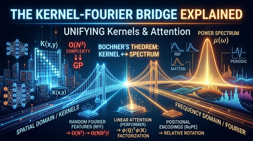
Level: Intermediate | Part 2 of artifocial W38 Basics | Research area: Spectral methods in machine learning
Companion Notebooks
This article pairs with two notebooks. Fourier Features from Scratch builds random Fourier features from the theorem below, measures the approximation error against the exact kernel, and computes the neural tangent kernel before and after the feature map. FNet vs Attention vs GP Attention implements dot-product attention, FNet and kernel-regression attention side by side and compares them on accuracy, scaling, and knowing-what-they-do-not-know. Both are pure NumPy and Matplotlib, CPU-only, with hand-derived gradients checked against finite differences, and both ship fully executed.
The empirical tables and training measurements below come from those notebooks’ saved output — Python 3.14.5, NumPy 2.5.3, seeds in the code. Algebraic examples are derivations, not additional experiments. The notebooks do not implement RoPE, FoPE, FAST, or a full spectral transformer.
Most practitioners meet kernels as a menu. You need a similarity function, you look at a list — RBF, Matérn, periodic, linear — you try two or three, and you pick whichever cross-validates best. It works, it is unsatisfying, and it gives you no way to answer the obvious question: what do I do when nothing on the menu fits?
Bochner's theorem replaces the menu with a construction. It says that continuous stationary positive-definite kernels normalized to correspond to probability measures over frequencies, and the correspondence is the Fourier transform. Once you believe that, choosing a kernel becomes drawing a picture of which frequencies your data contains, and the kernel is whatever the transform of that picture happens to be. You are no longer choosing from a list. You are specifying a spectrum.
That is the practical payoff, and this piece is mostly about earning it. The theorem also has three consequences that matter well beyond Gaussian processes: it explains why random Fourier features work, it explains what positional encodings are doing, and it puts attention and the FFT into the same family rather than adjacent chapters.
If kernels are new to you, Gaussian Processes Explained from W28 is the gentler entry point, and Attention Is a Kernel is the piece this one extends. This week's flagship, The Frequency Domain, takes the same lens across twelve weeks of tutorials.
What a kernel has to be
A kernel is a similarity score between two inputs. Not every function of two arguments qualifies, and the constraint is not a technicality.
The requirement is positive definiteness: for any finite set of points , the Gram matrix must be symmetric and have no negative eigenvalues for a real-valued kernel. Here “positive definite” follows the usual kernel-theory terminology and allows positive-semidefinite Gram matrices. The reason this is non-negotiable is that a kernel is implicitly promising the existence of a feature map with , and an inner product cannot produce an indefinite Gram matrix. Break positive definiteness and downstream machinery breaks with it: a Gaussian process's predictive variance can go negative, an SVM's optimisation stops being convex, a Cholesky factorisation fails outright.
The trouble is that positive definiteness is hard to check by inspection. It is a statement about every finite subset of the input space, quantified over all of them. Writing down a plausible-looking similarity function and verifying it is a legal kernel is genuinely difficult — which is a large part of why practitioners use the menu.
A stationary kernel depends only on the difference between its arguments: . Similarity depends on how far apart two points are, not where they are. Most of the standard menu is stationary, and this is the class Bochner's theorem describes.
The theorem
Bochner's theorem. A continuous positive-definite function on has a representation by a finite non-negative spectral measure : Conversely, every such measure defines a continuous positive-definite stationary kernel. Its total mass is , so normalizing makes a probability measure.
A density exists only when . Point masses are allowed too: a cosine kernel has atoms at a pair of frequencies. For a real-valued kernel, use a symmetric measure so the imaginary parts cancel. Then
for the normalized case. A non-unit kernel amplitude multiplies this expectation by .
Frequency convention. This article's equations use angular frequency and . The Fourier basic and parts of NB00 use cycles per unit, , and . They agree through . For an RBF of lengthscale , angular-frequency standard deviation is ; cycles-per-unit standard deviation is . Keep this factor when moving between the equations and code.
Read it slowly, because this is the whole article. A kernel is not merely related to a frequency distribution. It is one, transformed. The two objects carry identical information and you can move between them freely.
Why the "if and only if" is the useful part
Both directions do work.
Forwards, any probability distribution over frequencies gives you a valid kernel, automatically. You never have to verify positive definiteness again — you get it for free by construction, because the transform of a non-negative measure is positive definite. This is what turns kernel design from verification into specification.
Backwards, a stationary function whose Fourier transform goes negative anywhere is not a kernel, no matter how sensible it looks. This half has teeth, and the notebook demonstrates it with the most natural wrong answer available.
Consider the box similarity: if , else . Points within a radius are similar, points outside are not. It is symmetric, it peaks at zero, it decays, and it is exactly what a reasonable person would write down first. Its Fourier transform is a sinc function, which oscillates and goes negative — the notebook measures a minimum of −0.4338. (Strictly, the box's discontinuity is what puts it outside the theorem's continuity hypothesis — which names the hypothesis it fails, not the reason it is not a kernel. The reason is positive definiteness: the negative transform is the diagnosis and the Gram matrix below is the direct confirmation, and an indefinite Gram matrix disqualifies a candidate regardless of which hypothesis it sits outside.) So the transform says it is not a kernel, and we check: the Gram matrix of the box function on 40 points has a smallest eigenvalue of −3.4230, comfortably indefinite.
That is the theorem earning its keep. It told us the object was broken before we built a matrix, from a property of its transform, and it told us for a reason rather than by exhibiting a counterexample. It cannot serve as a valid GP covariance on all input sets. Particular calculations may fail factorization or yield invalid variances; this counterexample does not say every prediction is negative.
For contrast, the notebook verifies two kernels that do work. The RBF's spectral density matches its closed form to within and has a minimum of — zero, to numerical precision. The Matérn-1/2 (Laplace) kernel transforms to the Cauchy density, agrees with the closed form to under numerical integration, and has a strictly positive minimum. Non-negative densities, valid kernels.
Reading the standard menu as a spectrum
With the theorem in hand, the familiar kernels stop being arbitrary and start being statements about bandwidth.
RBF / squared-exponential. has a Gaussian spectral density with standard deviation . A Gaussian has extremely light tails, so the RBF says: essentially no energy beyond a soft cutoff. Not a hard band limit — a Gaussian density has full support, and the truly band-limited kernel is the sinc — but the spectrum dies faster than any polynomial, which is why GPs with RBF kernels produce famously, sometimes implausibly, smooth functions. A long lengthscale means a narrow density means only low frequencies, and the prior is smoother still.
Matérn. with smoothness has a Student-t spectral density, whose tails are polynomial rather than Gaussian. Heavy tails mean genuine high-frequency content is permitted, which is why Matérn kernels produce rougher, more realistic sample paths and why they are the better default for physical data. Choosing is choosing how fast the spectrum may decay — how much roughness you are willing to believe in.
Periodic kernels. A spectral measure concentrated at one frequency and its harmonics — deltas rather than a smooth density. Of course: that is what periodicity is.
White noise. A flat spectrum — all frequencies equally, no correlation at any lag. (A limiting case rather than a member: a flat "density" is not normalisable and the delta kernel is not continuous, so white noise sits at the boundary of the theorem's statement, the way physicists use it, not inside it.)
Notice what has happened to the menu. "Which kernel should I use?" was a question with no principled answer. "What frequency content does my data plausibly have, and how fast should the spectrum decay?" is a question a domain expert can answer, and it determines the kernel.
Designing off the menu
Once you are specifying the density, you can specify one that has no name.
The spectral mixture kernel (Wilson & Adams, ICML 2013) models as a symmetric mixture of Gaussians and takes the transform. Flexible mixtures approximate spectral densities, and narrow components can approximate atoms over a bounded lag range. This gives a trainable kernel family, but fitting its frequencies, weights, and widths is a nonconvex model-selection problem, not a guarantee of discovering the true spectrum.
What that buys you is automatic discovery of periodicity. Fit a spectral mixture kernel to a time series and the fitted nonzero component means propose frequencies, whose reciprocals are candidate periods. Held-out validation is still needed. You did not have to know they were there or specify them in advance. The notebook runs the construction in the clean direction: it places components at and cycles per unit, takes the numerical transform of the resulting kernel, and recovers peaks at exactly and .
It also shows the honest caveat. The recovered spectrum carries smaller ripples flanking each peak, which are not structure — they are spectral leakage from truncating the domain to a finite window, the uncertainty principle appearing as a measurement artefact. If you are reading fitted spectral components as discovered periods, you need to know which peaks are real, and the answer depends on your window rather than on your data.
Random Fourier features: the theorem as an algorithm
Kernel methods have a scaling problem. Exact GP inference needs the Gram matrix and a factorisation of it: memory and time. That is fine at and impossible at .
Bochner's theorem provides one standard approximation, and the derivation is two lines. The theorem says
The right-hand side is an expectation, and expectations can be estimated by sampling. Draw frequencies from , expand the cosine of a difference into a product, and you get an explicit feature map:
with . Here we assume the normalized kernel and sample from its spectral probability measure; multiply features by for a different amplitude. This is Rahimi and Recht's construction, and the entire content of it is "Bochner said this was an expectation, so let us sample it."
The random phase is not decoration
The one step that is easy to copy without understanding is the offset , so it is worth a paragraph.
The obvious way to turn into an inner product is the angle-difference identity:
which gives the two-component feature per sampled frequency. That works, and it is what the notebook's map uses. The cost is that frequencies produce features.
The single-component alternative uses a product-to-sum identity instead. With a random phase drawn uniformly on the circle,
because the second cosine, whose argument is uniformly distributed around the circle, averages to exactly zero. The random phase is what kills the unwanted term, and it is why the factor is rather than .
Both constructions estimate the same kernel, but must be counted consistently: paired frequencies use features, while random-phase cosines use . For the paired map, divide the concatenated vector by when estimating a unit-amplitude kernel. The reason is visible at zero lag: each frequency contributes to the squared norm, so the unnormalized inner product returns rather than , and the is what puts the estimator on the kernel's own scale rather than times it. The unnormalized used as neural-network input is a separate scaling choice.
What this buys in GP inference, concretely
The speed-up is worth spelling out because it changes the shape of the computation, not just its constant.
Exact GP regression solves with of size : the function-space view, . Substitute with of size and the Woodbury identity converts it into a problem — the weight-space view — costing . For large and smaller , that can be a substantial reduction, but it is not a runtime prediction. Forming the sufficient statistics still costs , and storing all features costs unless we stream them.
Two things survive the substitution and one does not. You keep the predictive mean and, importantly, the predictive variance in closed form: the approximation is a finite-dimensional Bayesian linear regression, which has the same posterior machinery. You also keep the ability to update online, since the sufficient statistics accumulate. What you lose is exactness at long range: the finite feature set makes the effective kernel slightly wrong, and the error shows up most where the data is sparse — which is precisely where the predictive variance is doing its most important work. Validate the approximate posterior against the original kernel where feasible, including sparse and extrapolation regions; location inside the training range is not a calibration guarantee.
The consequence is a change of cost class. Instead of an implicit kernel requiring an matrix, you have an explicit -dimensional feature map and can run linear methods on the transformed data. A pass of a linear-model optimizer costs roughly after feature construction; the exact finite-feature Bayesian solve above costs . These are different algorithms, and feature generation also depends on input dimension.
How good is the approximation
Monte Carlo error falls like , and it is worth checking that rather than assuming it. The notebook approximates an RBF kernel on 200 points in four dimensions, averaged over five draws:
| max abs error | rms error | ||
|---|---|---|---|
| 16 | 0.46363 | 0.22918 | 0.25000 |
| 64 | 0.27045 | 0.12362 | 0.12500 |
| 256 | 0.13427 | 0.06244 | 0.06250 |
| 1,024 | 0.05861 | 0.03043 | 0.03125 |
| 4,096 | 0.03595 | 0.01570 | 0.01562 |
| 16,384 | 0.01512 | 0.00724 | 0.00781 |
The fitted log-log slope is −0.498 against a theoretical −0.500.
Two practical readings. First, the rate is genuinely , which means halving your error costs four times the features. Do not plan on driving this error to zero; plan on choosing a tolerance. Second, the constant is friendly: at the observed RMS error is 0.06244 and maximum error 0.13427 on a kernel whose values live in , which is why the method is used in practice rather than admired in papers.
The bridge to positional encodings
Here is the connection that surprises people, and it is one line.
A positional encoding — the sinusoids-at-many-frequencies map that transformers apply to positions, and that coordinate networks apply to — has exactly the form of above. Sines and cosines of the input at a range of frequencies.
For a paired sine–cosine map with fixed frequencies, its inner product is exactly a stationary finite-spectrum kernel. It approximates a separate target kernel only if we specify a sampling or quadrature construction for that target. NeRF’s octave-spaced encoding chooses a deterministic bank; Tancik et al. sample it from a Gaussian; the difference is a sampling scheme, not a different idea.
This reframes a hyperparameter that otherwise looks arbitrary. "How many frequency bands, and how wide?" is not a design question about encodings. It is the question "what bandwidth should my implicit kernel have?" — which is the same question as choosing a lengthscale, and you already know how to think about that.
The first notebook makes the claim concrete rather than rhetorical. A plain two-hidden-layer MLP fitting recovers 100.3% of the slow component's amplitude and 25.6% of the fast one, after the recorded 4,000 steps. A model with the same hidden widths fed recovers 99.8%. Its wider input raises the parameter count from 16,897 to 33,153. NB00 also checks a 33,121-parameter plain control, which recovers 24.0%; that is the relevant control for a parameter-count explanation.
The mechanism is the kernel, and the notebook measures it directly. In the wide limit a network trained by gradient descent behaves like kernel regression with its neural tangent kernel, which for a one-hidden-layer ReLU network has a closed form — the notebook evaluates that form as an analytic proxy for the two-hidden-layer network it trains. On the raw coordinate that kernel has a measured stationarity error of 0.8486 and a half-width of 0.5354 — broad, and depending on absolute position rather than only on distance. On it becomes 0.0864 and 0.0236: narrow and, to a good approximation, stationary. The raw kernel is eight full periods of the target's fast component wide, consistent with a bias against learning it quickly, not a proof that it cannot represent it; the feature map brings it to about a third of a period.
The exact identity concerns the feature inner product. Relating it to a trained neural network adds architecture and training-limit assumptions. The analytic one-hidden-layer kernel here is a mechanism probe, not the measured empirical tangent kernel of the trained two-hidden-layer network — and the trained network's own kernel spectrum may differ from the proxy's in width, in stationarity, and in how it moves during training, none of which we measured.
Rotary positions: phase matters beyond a feature dot product
The flagship now asks which transformer components already use frequency structure. RoPE is a useful case because we can derive the core relation without conflating it with a stationary attention kernel. For one two-dimensional query/key pair, let be a rotation. At positions and ,
The absolute rotations combine into a relative angle. Multiple coordinate pairs use different frequencies. Unlike adding a fixed positional feature vector, RoPE rotates content-bearing query and key coordinates before their dot product. The score still depends on and : the identity does not turn a content-adaptive attention matrix into one fixed stationary convolution.
The FoPE paper studies this construction through discrete signal processing and argues that surrounding linear layers, nonlinearities, and insufficiently trained frequencies can impair length generalization. Its Fourier-series construction reports improvements under the tested settings. That is evidence about a particular position-encoding method, not proof that every interface between a learned representation and a Fourier representation destroys information.
The useful question for implementation is where phase, amplitude, and sampling range change. A full invertible FFT loses nothing merely by changing basis. Dropping phase, truncating modes, quantizing coefficients, or imposing an unsuitable periodic boundary can lose information. Name the actual operation before blaming “the interface.” This is the bridge from the basic theorem to the flagship's component audit.
Attention, and the last link in the chain
W28 established that attention is kernel regression. Softmax attention computes
which is the Nadaraya–Watson estimator with an exponentiated dot-product kernel.
Bochner adds the next link. Swap for a stationary kernel — an RBF, say — and the theorem applies: that kernel is an expectation over Fourier features. A stationary kernel score admits a spectral-feature representation. That does not imply an FFT implementation: stationarity in learned feature coordinates is different from shift invariance along sequence positions.
The second notebook makes this a two-line code change and then measures what it costs. Its mix() function implements dot-product attention and RBF kernel-regression attention with the same surrounding block, the same optimiser, the same seed; the only difference is the scoring function. Both reach 1.000 on the notebook's content-routing task and 0.999 on the global-structure task. The accuracy is similar in this run; the runtime table does not show identical computational cost.
This also makes the linear-attention literature legible. If for an explicit feature map, then
and the inner sum does not depend on . Compute it once and attention costs instead of — linear in sequence length. Performer uses positive orthogonal random features to approximate softmax attention. Random Feature Attention develops related random-feature approximations. They share the factorization strategy; it is inaccurate to identify all of their features with ordinary sine–cosine Bochner features. For softmax, the identity
exposes an RBF factor and norm-dependent factors. It is completing the square and nothing more: , so , and exponentiating splits that sum into the three factors above. Those factors and the chosen estimator matter. For normalized attention we must also approximate in the denominator. Signed Fourier estimates can make that denominator unstable; small kernel approximation error alone is not enough to certify an attention implementation.
What the bridge does not carry
A synthesis is only useful if it is honest about its limits, and there are three worth stating.
Bochner is about stationary kernels only. The dot-product kernel inside standard attention is not stationary — depends on the vectors, not on their difference — so the theorem does not apply to vanilla attention directly. What applies is the weaker and still useful statement: attention is kernel regression, and if you choose a stationary kernel, Bochner then applies to that choice. Under its regularity and domain assumptions, Mercer’s theorem provides an eigenfunction expansion for a positive-definite kernel rather than a frequency distribution; it is not the definition of positive definiteness, and those eigenfunctions coincide with Fourier modes only when the kernel is stationary on a domain with the right symmetry.
"Spectrum" means two different things in this area. The spectral density of Bochner's theorem is a distribution over frequencies obtained by Fourier transform. The spectrum of a matrix is its set of eigenvalues. Spectral normalization constrains a weight matrix’s largest singular value; spectral radius concerns its eigenvalues. Neither is generally a Fourier-frequency statement; the spectral bias of a neural network (Rahaman et al., arXiv:1806.08734; this week's companion explainer) is a frequency statement. The two coincide only when the operator in question commutes with a translation symmetry — which is exactly when its eigenvectors are Fourier modes, and that is a condition to check rather than assume. Conflating them is the easiest available mistake in a piece like this one.
The uncertainty story needs a qualifier. It is often said that the kernel view gives you principled uncertainty for free. The second notebook tested that directly and the result is more interesting than the slogan. On an out-of-distribution test — a query whose matching key is absent, so the routing question has no answer — all three models drop to chance, but the measured signals from the content-dependent models separate the two sets better in this experiment. The closed-form GP posterior variance, the principled answer, reaches an AUROC of just 0.657 even after sweeping the lengthscale over six values and reporting the best. The peak routing weight — a crude read of how much attention mass landed on any single slot — separates the two sets perfectly, at 1.000, and plain dot-product attention does it just as well as the RBF version.
One interpretation of this result is worth testing further. The posterior variance measures how well the query is covered by the key set as a whole, and sixty-three keys at moderate distance provide about as much coverage whether or not one is an exact match — so the discriminating information gets averaged away. The softmax normalises, so what survives is the contrast between the best key and the rest, which is precisely where the routing signal lives. An absolute quantity washed it out; a relative one recovered it exactly.
The lesson is not that Gaussian processes do not give uncertainty. It is that "it is a GP so it has principled error bars" is not a measurement, and you have to ask which functional of the kernel you are reading and check it against the failure you actually care about.
For comparison, the same notebook's FFT-mixing model scores 0.495 — a coin flip — on the same test, in this saved experiment. That is not an impossibility theorem for deeper nonlinear architectures containing Fourier mixers. FNet has no data-dependent weights anywhere in its mixer, so there is no routing distribution to interrogate. A fixed mixer supplies no learned routing distribution to inspect. This does not rule out other OOD detectors or uncertainties built around its representation.
Beyond the real line: the same theorem on other spaces
One reason to trust this correspondence rather than treat it as a coincidence of Euclidean space is that it generalises, and the generalisation explains several constructions that otherwise look unrelated.
The deep statement is that the Fourier basis is not arbitrary. It is the set of functions that diagonalise translation — the characters of the group of shifts. Change the symmetry group and the same construction produces a different basis, and stationary kernels on that space decompose in it.
On the sphere, the symmetry is rotation and the basis is spherical harmonics. A rotation-invariant kernel on the sphere is a non-negative weighting of harmonic degrees, and truncating to low degree is a bandwidth choice. This is exactly what the spherical-harmonic colour representation in 3D Gaussian Splatting is doing: capping the harmonic order caps how sharply appearance may vary with viewing angle. Same theorem, different group.
On an undirected graph, a symmetric graph Laplacian has an orthonormal eigenbasis, often called the graph Fourier basis. If , choosing gives a positive-semidefinite kernel . A graph-distance similarity is not automatically a function of the Laplacian or a valid kernel. Spectral graph neural networks are built directly on this, and the familiar warning that they transfer badly between graphs is the statement that the basis itself is graph-dependent — the "frequencies" are not the same objects across two different graphs.
On a general compact group, the Peter–Weyl theorem provides the basis: the matrix entries of irreducible representations. Equivariant networks that convolve in "irrep space" are applying the convolution theorem in that basis, for the same reason and with costs that depend on the group and implementation; a Euclidean FFT complexity bound does not automatically transfer.
The practical value of knowing this is mostly one of orientation. When you meet a new equivariant or geometric architecture, the useful first question is which symmetry group is being assumed, and what is the induced basis — because the answer tells you what the model can represent cheaply and what it cannot represent at all.
Reading the spectral-transformer audit without collapsing the categories
The flagship's expanded audit includes encodings, mixers, and outputs. Bochner gives us a precise way to sort them rather than calling everything “frequency-domain attention.”
Read the table as a taxonomy, not a benchmark. The right-hand column is what each construction leaves for you to check, and it carries no numbers deliberately: our notebooks implement paired Fourier features and FFT mixing only, so RoPE, random-feature attention, FNO and FAST stand here on their citations and not on anything we measured. Anyone quoting an impact figure for them should take it from the cited paper under that paper's conditions.
| Construction | What it changes | What we still need to check |
|---|---|---|
| Paired Fourier features | Input coordinates and their induced kernel | Frequency convention, scale, feature budget |
| RoPE | Position-dependent phase of queries and keys | Training range and content-dependent scores |
| FFT token mixing | How positions and hidden coordinates are mixed | Phase loss, boundary assumptions, whole-block cost |
| Random-feature attention | Approximation of a kernel-weighted numerator and denominator | Variance, positivity, denominator stability |
| Fourier neural operator | Learned transformations of spatial modes | Boundary conditions, truncation, resolution transfer |
| Frequency-based action tokenization | Representation of a sampled action sequence | Quantization and reconstruction error |
For the final row, FAST applies a discrete cosine transform in a compression-based robot-action tokenizer. Its frequency axis is time across an action chunk. That is an input/output representation decision, not a replacement for the transformer's content-routing mechanism. It illustrates why spectral methods can help where the signal axis has a concrete interpretation.
For the neural-operator row, the FNO paper parameterizes operators in Fourier space. A learned frequency multiplier need not be non-negative and need not define a covariance kernel. Bochner’s positivity requirement applies when we claim a valid stationary covariance, not to every trainable spectral filter.
Likewise, the Fourier basis diagonalizes a linear convolution on the corresponding periodic grid; it does not diagonalize every content-dependent network. A nonlinear model can combine fixed spectral mixing with learned layers and become content-dependent overall. Our notebook’s single-block routing result therefore supports a specific architectural comparison, not a theorem forbidding frequency-based language models. The full-stack research question remains empirical: compare task quality, retained information, and measured cost under matched conditions.
The whole chain in one place
Read these arrows with their conditions: stationary positive-definite kernels for Bochner, explicit sampling choices for RFF, a GP model for posterior variance, and stable normalization for attention. The notebook checks selected links; it does not validate every spectral architecture. What the chain buys is that a technique you already use in one place tells you something about a technique you use in another: tuning an encoding bandwidth and choosing a GP lengthscale are the same act, and the intuition transfers.
Checklist
- Specify the spectrum, not the kernel. Ask what frequency content your data plausibly has and how fast the spectrum should decay. That determines the kernel; the menu was only ever a shortcut.
- A plausible similarity function needs a validity argument. For a continuous stationary candidate, a non-negative spectral measure supplies one. A finite numerical Fourier grid or a few Gram matrices alone cannot prove validity for every input set.
- Read lengthscale as bandwidth. Long lengthscale means a narrow spectral density means a low-pass prior. Short means the opposite. Matérn over RBF when you believe there is genuine roughness — the tails of the density are the whole difference.
- Budget RFF features against a tolerance, not against zero. The error falls as , so halving it costs four times the features.
- Treat a positional encoding as a kernel choice. "How many bands and how wide" is "what bandwidth should my implicit kernel have", and you have priors about that.
- Fit a spectral mixture kernel when you suspect unknown periodicity — a nonzero component mean identifies a frequency, whose reciprocal is a candidate period. Validate it against held-out data and alternative fits. Check the ripples around each peak against your window length before believing them.
- Say which spectrum you mean. Frequency-domain and eigenvalue statements coincide only when the operator commutes with a translation symmetry.
- Name the uncertainty functional. "It is a GP" is not an uncertainty estimate. Pick the functional, then measure it against the failure you care about — the principled one is not automatically the discriminating one.
Sources
- Random Features for Large-Scale Kernel Machines (Rahimi & Recht, NeurIPS 2007)
- Gaussian Process Kernels for Pattern Discovery and Extrapolation (Wilson & Adams, ICML 2013)
- Fourier Features Let Networks Learn High Frequency Functions in Low Dimensional Domains (Tancik et al., arXiv:2006.10739)
- On the Spectral Bias of Neural Networks (Rahaman et al., arXiv:1806.08734)
- FNet: Mixing Tokens with Fourier Transforms (Lee-Thorp et al., arXiv:2105.03824)
Our own earlier pieces this one builds on: Attention Is a Kernel · Gaussian Processes Explained · Why Uncertainty Matters
We build agent systems and practitioner tooling at Artifocial — see our apps, including Alarmly.