Fourier Transforms Explained: From Signals to Spectral Bias

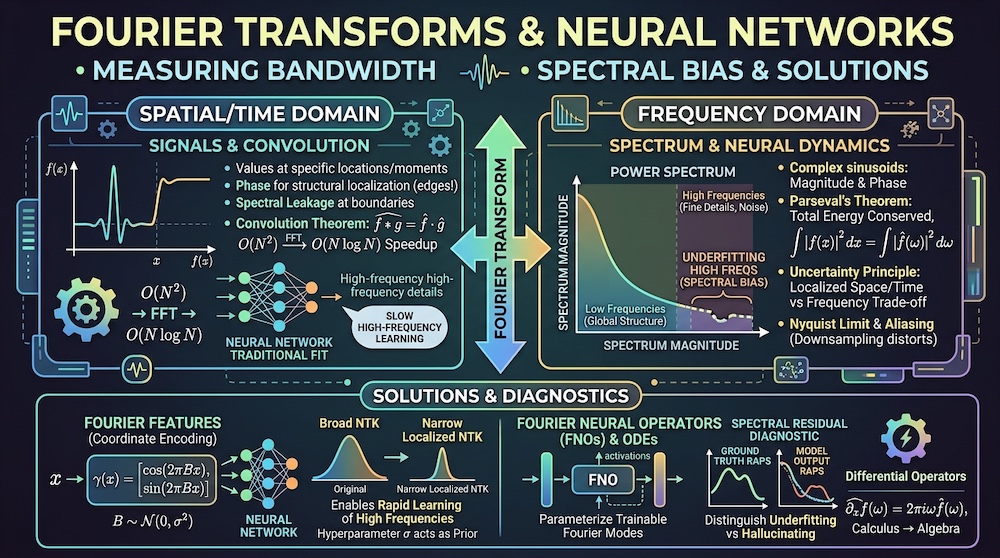
Level: Intermediate | Part 1 of artifocial W38 Basics | Research area: Spectral methods in machine learning

Companion Notebook

This article pairs with Fourier Features from Scratch — pure NumPy and Matplotlib, CPU-only, running top to bottom in about a minute with every figure inline and the MLP's backward pass written out by hand. It carries the same material in runnable form: a two-tone target whose spectrum is exactly known, a plain MLP that recovers 100.3% of the slow component and 25.6% of the fast one, random Fourier features verified against the $D^{-1/2}$ rate, Bochner's theorem checked in both directions including a function that is not a kernel, and the neural tangent kernel computed directly before and after the feature map.

The training and kernel measurements below come from that notebook's saved output. The timing and normalization examples come from FNet vs Attention vs GP Attention. Both record Python 3.14.5, NumPy 2.5.3, and their seeds. Worked arithmetic is labeled separately; these CPU demonstrations are not production benchmarks.

Most explanations of the Fourier transform start with music. A chord is several notes at once; the transform tells you which notes. That is a true and useless place to start if what you actually want is to know why your model will not learn sharp edges.

So this piece starts somewhere else: with the observation that a neural network trained by gradient descent has a bandwidth, that the bandwidth is a real measurable quantity, and that almost everything practitioners find confusing about high-frequency detail becomes obvious once you can measure it. The Fourier transform is the tool that makes it measurable. The music is a side effect.

This is the ground floor for this two-week's flagship, The Frequency Domain, which takes the same lens across twelve weeks of our tutorials. Read this one first if the phrase "spectral density" does not already mean something specific to you.

Why change the representation at all?

The newer flagship starts with a familiar engineering move: put the data into coordinates where the operation we need becomes easier. Learned word embeddings make some relationships accessible through dot products. A Fourier transform exposes repeated structure through sinusoidal coefficients. Both change the representation, but they make different promises.

An embedding is learned from examples and a training objective. Its usefulness depends on that training, and it need not preserve enough information to reconstruct its input. A complete DFT is a fixed, invertible linear map. It needs no training and preserves the samples, up to numerical roundoff. Neither property guarantees that its coordinates are the best ones for the task. An invertible rearrangement of a difficult problem can still be difficult.

The practical test is therefore not “can we Fourier-transform this?” Almost any sampled array qualifies. It is “does the operation become simpler?” A shift changes phase predictably; a convolution becomes multiplication. Those identities provide computational benefits. Transforming an arbitrary ordering of vocabulary IDs provides no comparable semantics: adjacent IDs need not denote related words. Even the hidden dimensions of a learned embedding can be reordered without changing its information, so a DFT over those dimensions is a mixing operation, not automatically a physically interpretable spectrum.

That distinction will keep us from treating every Fourier-based neural layer as the same technique. A feature map changes what an MLP receives. An FFT mixer combines positions. A spectral diagnostic measures a prediction. They use related mathematics for different jobs.

Two ways to describe the same thing

A signal in the time domain (or space domain, for an image) is a list of values: what is happening at each moment or each pixel. A signal in the frequency domain is a different list: how much of each repeating pattern the signal contains, and where each pattern sits in its cycle.

Neither is more fundamental. They are two coordinate systems for the same object, and you can move between them without losing anything. The reason to bother moving is that questions which are hard in one are sometimes trivial in the other.

The canonical example: "does this signal repeat with a period of about a second?" In the time domain that is a search problem — you would slide a window along and correlate. In the frequency domain it is a lookup: go to the bin at 1 Hz and read the number. Conversely, "when exactly did the loud part happen?" is trivial in time and awkward in frequency. Choosing the domain is most of the work.

For a function $f$ on the real line, the transform and its inverse are

\hat{f}(\omega)=\int_{-\infty}^{\infty} f(x)\,e^{-2\pi i \omega x}\,dx, \qquad f(x)=\int_{-\infty}^{\infty} \hat{f}(\omega)\,e^{2\pi i \omega x}\,d\omega .

Read the first equation as a scoring procedure. To find out how much of frequency $\omega$ is in $f$ , multiply $f$ by a complex sinusoid at that frequency and add up the result. If $f$ contains that pattern, the product stays consistently positive in the right direction and the sum is large. If it does not, the product oscillates and cancels to nothing. The transform is a bank of matched filters, one per frequency, run all at once.

The complex exponential is doing two jobs. $e^{-2\pi i \omega x} = \cos(2\pi\omega x) - i\sin(2\pi\omega x)$ , so the real part measures overlap with a cosine and the imaginary part overlap with a sine. Together they give magnitude (how much of that frequency) and phase (where in its cycle it starts).

The smallest possible worked example

The matched-filter reading is worth making concrete once, because the four-point DFT can be done in your head and it makes the cancellation visible.

Take $N=4$ and the sample list $x = [1, 0, -1, 0]$ — one full cycle of a cosine sampled four times. The DFT basis at frequency $k$ evaluates $e^{-2\pi i k n/4}$ for $n = 0,1,2,3$ , which for $k=1$ is $[1, -i, -1, i]$ .

$X_0 = 1 + 0 - 1 + 0 = 0$ . The zero-frequency bin is the sum, i.e. $N$ times the mean. Our signal averages to zero, so there is no DC component.
$X_1 = (1)(1) + (0)(-i) + (-1)(-1) + (0)(i) = 1 + 1 = 2$ . The signal and the $k=1$ basis vector agree everywhere they are both non-zero, so the terms add instead of cancelling.
$X_2$ uses the basis $[1, -1, 1, -1]$ : $1 - 0 - 1 - 0 = 0$ .
$X_3$ uses $[1, i, -1, -i]$ and gives $2$ , the mirror of $X_1$ .

Three things fall out of five lines of arithmetic. The energy landed entirely in the bin corresponding to the frequency actually present, which is the matched filter working. The result is real rather than complex, because our signal is an even cosine with zero phase offset — shift the samples to $[0, 1, 0, -1]$ and the same magnitudes reappear with the values rotated into the imaginary axis. And $X_3$ mirrors $X_1$ , which is the general fact that the DFT of a real signal is conjugate-symmetric: the second half of the output carries no new information, which is why np.fft.rfft returns only $\lfloor N/2 \rfloor + 1$ values and why you should use it rather than discarding half of a full transform by hand.

Phase is not the boring half

Practitioners routinely plot magnitude and throw phase away. That is fine for asking "what frequencies are present" and misleading in a specific way worth knowing about.

The standard demonstration: take two photographs, transform both, then recombine the magnitudes of the first with the phases of the second and invert. The result looks like the second image. Phase carries the alignment information — where each frequency component sits — and alignment is what makes edges line up into objects. Magnitude alone tells you a scene contains a lot of energy at a particular scale and nothing whatever about where.

This has a direct consequence for evaluation. A metric computed on magnitude spectra alone — including the radially averaged power spectrum recommended later in this piece — is blind to a model that puts the right amount of energy in the right bands and in the wrong places. That is not a reason to avoid the diagnostic; it is a reason to pair it with a spatial one. Spectral comparison catches the failures that pixel error hides, and pixel error catches the failures that spectral comparison hides. Neither subsumes the other, which is why the recommendation below is to plot the ratio of two spectra alongside your existing loss rather than instead of it.

Periodic versus not: series versus transform

If your signal repeats exactly, only frequencies that fit a whole number of times into one period can contribute, so the spectrum is a discrete set of spikes and the decomposition is a Fourier series. If it does not repeat, every frequency can contribute a little and the spectrum is a continuous curve — the Fourier transform proper.

This distinction matters in practice for one reason. When you take the DFT of a finite chunk of data, you are implicitly claiming the data repeats with a period equal to your window. It almost never does, so the value at the end of your window does not match the value at the start, and that artificial jump has energy at every frequency. This is spectral leakage, and which is why spectral estimation often uses a taper before transforming. A taper reduces sidelobes at the cost of broader peaks; it is a choice, not a requirement for an exactly periodic, bin-aligned signal.

You can watch it happen in the notebook: the spectral mixture kernel there is designed with components at $\omega = 0$ and $\omega = 1.5$ , and the numerical transform recovers exactly those two peaks — along with a family of smaller ripples either side which are pure leakage from truncating the domain to $[-8, 8]$ . Nothing is wrong with the code. The ripples are the price of a finite window, and recognising them as an artefact rather than as structure is a skill worth having before you start reading spectra of your own data.

The three properties that do all the work

Textbooks list a dozen properties. In machine learning, three of them carry essentially the entire load.

Linearity

The transform of a sum is the sum of the transforms, and scaling the input scales the output. Unexciting, and the reason everything else composes: you can analyse the frequency content of a sum of effects one effect at a time.

The convolution theorem

This is the load-bearing one:

$\widehat{(f * g)}(\omega) = \hat{f}(\omega)\,\hat{g}(\omega).$

Convolution in one domain is pointwise multiplication in the other. Direct convolution of two length- $N$ signals costs $O(N^2)$ ; a short length- $K$ filter instead costs $O(NK)$ . Pointwise multiplication is $O(N)$ . Since the transform itself costs $O(N \log N)$ (next section), you can convolve two long signals by transforming both, multiplying, and transforming back, for $O(N \log N)$ total. For linear convolution, pad to at least the sum of the input lengths minus one; an unpadded DFT product computes circular convolution.

Two consequences worth carrying:

Filtering is easy in frequency space. A low-pass filter in the time domain is a convolution with some carefully-shaped kernel. In the frequency domain it is: multiply the high-frequency bins by zero. Blurring, sharpening, and band-limiting are all one-line operations once you are in the right basis. One caveat: zeroing bins outright is the ideal ("brick-wall") low-pass, and its time-domain counterpart is the slowly-decaying sinc — so a hard cutoff buys you ringing (Gibbs oscillations) around any sharp edge in the signal. Practical filters trade a gentler frequency roll-off for less ringing; the one-liner is the concept, not the production filter.

Every quadratic all-pairs operation deserves the question "is this a convolution?" If the answer is yes — if the interaction between two positions depends only on the distance between them — the FFT is available and the cost drops. This question is the entire origin of the FFT-based architectures the flagship covers.

Parseval's theorem

Total energy is preserved:

$\int |f(x)|^2 dx = \int |\hat{f}(\omega)|^2 d\omega .$

The transform is a rotation of the space, not a distortion of it. Nothing is created or destroyed, which is what makes "transform, work, transform back" an exact procedure rather than an approximation.

Parseval also licenses the most useful diagnostic in this article. Because energy is conserved, you can ask where in the spectrum a model's error lives, and the answer partitions the total error exactly. We return to this below.

There is a practical corollary that the notebook runs into directly. The DFT has several conventions for where the normalisation constant goes, and the one that makes Parseval hold exactly is the unitary or orthonormal DFT, with a $1/\sqrt{N}$ on each transform. Use the unnormalised convention inside a neural network layer and the activation energy is inflated by the product of the transform lengths — in the second notebook's setup (01_fnet_vs_attention_vs_gpa.ipynb), a factor of about 2,048. Amplitudes scale as the square root of energy, so that is a measured rms jump from 0.46 to 15.02 — about 33× once taking the real part discards half the energy — and it saturates everything downstream. The fix is either a normalisation layer or the unitary convention, both control activation scale. They are not identical operations: unitary scaling is a fixed linear factor, while LayerNorm depends on each activation vector. Taking only the real part still discards information; normalization does not restore it.

The uncertainty principle, and why it constrains your tools

One constraint deserves more prominence than it usually gets: a signal cannot be sharply localised in both position and frequency. Narrow in time means broad in frequency; narrow in frequency means broad in time.

This is not a physics fact with a signal-processing analogy attached. It is a theorem about Fourier pairs — quantum mechanics inherits it because position and momentum happen to be a Fourier pair. The reason it matters here is entirely practical.

A global spectrum does not locate changes in time. If your data is a recording that is quiet then loud, or a training run that behaves differently early and late, a single Fourier transform over the whole thing reports an average that may describe no part of it. The transform itself requires no stationarity assumption. Stationarity matters when we interpret one aggregate spectrum as a description of statistics that hold throughout the recording.

The response is to give up some frequency resolution to buy time resolution. The short-time Fourier transform chops the signal into overlapping windows and transforms each one, producing a spectrogram: frequency content as a function of time. The window length is the trade-off dial, and the uncertainty principle sets the exchange rate. Short windows localise events in time and blur nearby frequencies together; long windows separate frequencies finely and smear the timing.

Wavelets make the trade-off adaptively: short windows at high frequencies, long windows at low ones, on the reasonable prior that fast events are brief and slow structure persists. That is why JPEG 2000 uses them where the original JPEG used a block cosine transform, and why they won the niches where multi-scale detail matters most — digital cinema, medical imaging — even though most deployed image codecs remain DCT-based.

The practical rule is short. Before interpreting a global spectrum, ask whether its statistics are representative across the domain. If timing or changing statistics matter, add a spectrogram. The global transform remains valid; its summary may not answer the question we meant to ask.

Why audio and images use different spectral tools

The flagship's expanded audio–vision comparison has a useful foundation: a transform can simplify part of a generating process without explaining the whole modality. In a short voiced-speech segment, the source–filter approximation treats vocal excitation as passing through a vocal-tract filter. Convolution becomes multiplication in frequency, and logarithms turn that product into a sum wherever the magnitude is nonzero. This helps separate excitation structure from the spectral envelope. It is an approximation over a short interval, not a claim that a changing speaker is a single time-invariant system.

Time–frequency analysis also has a history independent of fast computation. The 1946 sound-spectrograph paper predates the 1965 Cooley–Tukey FFT paper. The FFT made digital transforms efficient; it did not invent the idea of examining speech in frequency bands. Today there are both spectrogram-based systems and learned waveform front ends. The signal-processing representation is useful, not compulsory.

For an image, optical blur can often be approximated by convolution, so frequency-domain deblurring has a direct mathematical justification. Object recognition is a different problem. Occlusion, shape, and the arrangement of parts do not reduce to a single global convolution. A magnitude spectrum can describe texture or coarse scene statistics, but it omits phase information that locates structure. The classic Oppenheim–Lim analysis explains why keeping phase matters when reconstructing recognizable images. This does not mean phase is irrelevant to audio; waveform reconstruction and timing-sensitive audio tasks can require it too.

This gives us a practical choice. For a sustained tone, a global spectrum may answer the question. For changing speech, use a time–frequency representation. For an image boundary, localized filters or patches retain spatial context. The question is which information the task needs us to preserve.

The DFT, the FFT, and what the speed actually buys

Real data is a finite list of samples, so we use the discrete Fourier transform:

$X_k=\sum_{n=0}^{N-1} x_n\, e^{-2\pi i k n / N}, \qquad k = 0, \ldots, N-1 .$

Computed directly this is $N$ sums of $N$ terms: $O(N^2)$ . The fast Fourier transform exploits the enormous redundancy among those complex exponentials — splitting even- and odd-indexed samples recursively — to get the same answer in $O(N \log N)$ .

The gap is not academic. At $N = 10^6$ , $N^2$ is $10^{12}$ and $N\log_2 N$ is about $2\times10^7$ : a factor of roughly fifty thousand. The FFT is a strong candidate for the most consequential algorithm of the twentieth century, and most of what follows in modern spectral methods exists because the transform is cheap.

Two caveats before you plan around the exponent.

Sampling sets a hard ceiling. A signal sampled $N$ times can represent frequencies only up to $N/2$ cycles across the window — the Nyquist limit. Content above that does not vanish; it folds back and appears as a spurious low frequency. This is aliasing, and it is the reason wagon wheels appear to spin backwards on film.

The folding rule is worth knowing precisely, because it lets you predict where a contaminant will land instead of discovering it. Sample at rate $f_s$ and a component at frequency $f$ above $f_s/2$ appears at $|f - k f_s|$ for whichever integer $k$ brings it into the band. Sample a 90 Hz tone at 100 Hz and it arrives as $|90 - 100| = 10$ Hz — a slow, clean, entirely fictitious oscillation, indistinguishable after the fact from a real one. Nothing downstream can undo this. The information was destroyed at the moment of sampling, and the alias is not noise you can average away; it is a well-behaved signal at the wrong frequency.

In machine learning this bites whenever you downsample without filtering first. Resize an image with nearest-neighbour or naive striding and the texture above the new Nyquist limit folds into low-frequency moiré that the model will faithfully learn as structure. It bites again in video: a deformation field reconstructed from frames at a given rate cannot represent motion faster than half that rate, so "the model struggles with fast motion" often has an exact quantitative form that no amount of training addresses. And it bites in the evaluation harness, where an aliased validation set can make a model look better than it is by removing exactly the high-frequency content the model was going to fail on. Low-pass filter before you decimate — that is the whole remedy, and it is one line in every imaging library.

A better asymptotic cost does not guarantee a faster block. The saved second-notebook run reports a whole-block FFT speed-up of 94.4× at sequence length 8,192, but 0.43× at length 64: slower at the shorter length. These are minimum-over-repetitions timings on one laptop CPU using NumPy's BLAS. They do not measure a GPU implementation or compare against fused production attention.

The constants-free ratio $N/\log_2 N$ is about 630 at 8,192. That is a comparison of growth terms, not a FLOP-count prediction of 630× speed-up: it omits feature width, constants, memory traffic, and the feed-forward work both blocks retain. Measure the complete workload at the lengths, batch sizes, precision, and hardware we intend to use. Record the mixer time separately so a fast subroutine does not masquerade as a fast model.

Where this starts mattering for neural networks

Everything so far is signal processing. Here is the bridge.

Many coordinate MLPs trained by gradient-based methods learn low frequencies before high ones. This is spectral bias, also studied as the Frequency Principle, and it is one of the more reliable empirical regularities in deep learning (Rahaman et al., arXiv:1806.08734).

It is easy to state and easy to demonstrate. The notebook fits a two-hidden-layer ReLU MLP to

$f(x) = \sin(2\pi x) + 0.3\sin(2\pi \cdot 15 x)$

a slow component at amplitude 1.0 and a fast one at amplitude 0.3. Because the target is a sum of sinusoids at integer frequencies on a uniform grid, its spectrum has exactly two non-zero bins and we know their heights exactly. That turns "the model got the coarse shape but not the detail" from an impression into a number.

After 4,000 full-batch Adam steps the width-128 network has recovered 100.3% of the slow component's amplitude and 25.6% of the fast one. At step 975 the fast amplitude was 0.0352, about 12% of its target 0.3. This establishes unequal progress within this run. It does not establish that more training can never work, nor justify extrapolating a convergence time from two checkpoints.

A useful explanation comes from kernel-style training dynamics: directions with small tangent-kernel eigenvalues can learn slowly. That is a local or limiting approximation, not a proof that a finite network trained with Adam follows fixed-kernel gradient flow. The result motivates a controlled representation change and a comparison against a larger plain model.

Why this is sometimes exactly what you want

Spectral bias is a free regulariser, and understanding that is half of using it well.

In some tasks, useful structure is concentrated at lower frequencies while noise has substantial high-frequency energy. In others, fine-scale structure is the signal and low-frequency drift is the noise. A model that fits low frequencies first is a model that fits signal before noise. This is one explanation for why early stopping can help in that regime — you are halting the model in the window where it has acquired the structure and not yet acquired the noise. It is also part of why heavily over-parameterised models generalise better than the classical bias–variance account predicts: the implicit bias of the optimiser, not the capacity of the model, is doing much of the regularising.

And why it is sometimes the whole problem

When the thing you are representing genuinely is high-frequency, spectral bias is not a helpful prior but the central obstacle. Sharp edges. Fine geometric detail on a surface. Texture. Short-wavelength periodic structure. In those regimes a network converges beautifully to a blurred version of your target and then sits there — as the 25.6% recovery illustrates within the recorded training budget.

This is why coordinate-based networks needed a fix before they could work at all. A network mapping $(x, y, z)$ to colour and density has to represent detail at a spatial scale far finer than a plain MLP will reach, and Fourier features offer one way to reduce the tendency toward over-smoothed fits.

The fix, in one sentence

The fix is to change the input, not the network. Replace the raw coordinate $x$ with

$\gamma(x) = \big[\cos(2\pi B x),\; \sin(2\pi B x)\big], \qquad B_j \sim \mathcal{N}(0, \sigma^2)$

and train the identical architecture. In the notebook this takes the high-frequency amplitude recovery from 25.6% to 99.8%, with the same hidden-layer width, optimizer, step count, and data. The input dimension changes, so the parameter count does too: 16,897 for the plain width-128 model versus 33,153 for the feature model. The notebook also trains a width-180 plain control with 33,121 parameters; it recovers 24.0% of the fast component. That control supports a representation benefit beyond merely adding parameters, within this experiment.

That is a large enough jump to be suspicious of, so the notebook also measures why it happens rather than asserting it. In the wide limit a network trained by gradient descent behaves like kernel regression with its neural tangent kernel, and for a one-hidden-layer ReLU network that kernel has a closed form you can evaluate directly — the notebook evaluates that one-hidden-layer form as an analytic proxy for the two-hidden-layer network it actually trains, so read the numbers as the mechanism in miniature rather than the trained model's exact kernel. On the raw coordinate it is broad and non-stationary — similarity between two inputs depends on where they are, not just how far apart, with a measured stationarity error of 0.8486 and a half-width of 0.5354, more than half the domain. On $\gamma(x)$ it becomes a narrow, nearly-stationary band: stationarity error 0.0864, half-width 0.0236. The raw-coordinate kernel is eight full periods of the target's fast component wide, which is consistent with slow learning of that component; width alone does not prove an expressivity limit. The feature map brings it to about a third of a period.

Fourier features are not a trick that happens to work. They change the kernel your network is implicitly doing regression with, and the change is measurable in about thirty lines.

The full story — why sampling frequencies from a distribution approximates a kernel, and what Bochner's theorem has to do with it — is in this week's companion explainer, Bochner's Theorem and the Kernel–Fourier Bridge.

The scale is a prior, and it cuts both ways

$\sigma$ , the spread of the sampled frequencies, is the dial. The notebook sweeps it and the NTK half-width falls from 0.1890 at $\sigma=1$ to 0.0630 at $\sigma=3$ to 0.0236 at $\sigma=10$ — narrower kernel, more capacity for detail, less implicit smoothing.

It is tempting to read that as "set $\sigma$ large." It is not. A kernel much narrower than the structure in your data fits the noise between your samples: the model interpolates the training points exactly and oscillates wildly in between. There is an interior optimum, and finding it is a real tuning problem rather than a monotone knob.

The sweep also illustrates a trap worth naming. Above $\sigma \approx 30$ the measured half-width stops moving, sitting at 0.0079 for both $\sigma=30$ and $\sigma=100$ . The tempting reading is "returns diminish past 30." The actual reason is that the statistic is computed on a 128-point grid and cannot report a width below one grid step, which is 0.0079. The measurement has bottomed out at its own resolution — which is a spatial-resolution limit of this width estimator, not a measured Nyquist cutoff of the model. A saturating instrument and a converged quantity print identically. The remedy is one line: print the instrument's floor next to the value.

The one diagnostic to take away

If you retain a single operational habit from this piece, make it this one.

Compare the power spectrum of your model's predictions against the power spectrum of the ground truth. For 2-D fields: FFT each, take the squared magnitude, and average over annuli of constant radius in frequency space so each bin is a spatial-frequency band regardless of orientation. Plot both curves on log axes, and plot their ratio.

The frequency at which the prediction curve falls away from the target curve is your model's effective bandwidth, and it is a far more actionable number than a validation loss. Agreement in power does not establish agreement in phase, and no sampled diagnostic establishes behavior beyond Nyquist. A shortfall well below Nyquist identifies a band to investigate. It does not by itself distinguish representation limits, optimization, regularization, or noise. Compare checkpoints and controlled changes before attributing the cause.

Run it across training checkpoints and you can watch the Frequency Principle happen: the crossover marches outward, quickly at first and then barely at all. The epoch at which it stops moving is a principled place to consider early stopping, and it is legible there long before validation loss flattens convincingly.

The reason this beats a scalar loss is Parseval. Squared error is the sum of the squared magnitudes of the residual spectrum under the unitary convention. Large low-frequency target power does not imply large low-frequency error. For an exact error decomposition, transform prediction minus target; subtracting their powers is not equivalent. Two very different failures produce the same MSE:

Underfitting high frequencies shows up as a prediction spectrum that decays too fast.
Hallucinating high frequencies — a model inventing texture that is not in the data, which is what over-scaled Fourier features do — shows up as a prediction spectrum with more energy than the target at high frequency.

They demand opposite fixes. A scalar cannot tell you which one you are looking at; three lines of NumPy can.

Differential equations: another reason to change basis

The newer flagship also connects Fourier methods to differential equations. Under suitable decay or periodic boundary conditions, differentiation in space satisfies

$\widehat{\partial_x f}(\omega)=2\pi i\omega\hat f(\omega).$

For a periodic heat equation $\partial_t u=\alpha\partial_{xx}u$ , each spatial Fourier coefficient therefore obeys

$\partial_t\hat u(\omega,t)=-4\pi^2\alpha\omega^2\hat u(\omega,t).$

This is worked algebra, not a notebook benchmark. A differential operator has become multiplication, and each mode decays independently. High frequencies decay faster. Boundary conditions and coefficients matter: variable coefficients or nonlinear products generally couple modes, so the same diagonal shortcut does not apply unchanged.

A Fourier Neural Operator learns transformations of Fourier modes inside a network, with other operations around the spectral layer. That differs from using Fourier features as inputs to an MLP that approximates a solution. The first changes a layer's operator; the second changes the coordinates seen by a function approximator. Neither makes difficult PDEs automatically solved, and neither experiment is implemented by this week's two notebooks.

Where you have already been using this

A short list, to make the point that this is not a specialist topic.

JPEG transforms 8×8 image blocks with a discrete cosine transform, then quantises high-frequency coefficients aggressively. It works because natural images are sparse in the frequency domain — most of the energy is in a few low-frequency coefficients — and because human vision is less sensitive to high-frequency error. Compression is a bandwidth decision made explicit.

Audio processing is frequency-domain almost end to end. MP3 discards frequency bands that psychoacoustic masking says you will not hear. Many speech models consume log-mel spectrograms: short-time spectral power aggregated through mel-spaced filters, then log-compressed. Others learn representations directly from waveforms.

Convolutional networks are, by the convolution theorem, applying learned frequency-selective filters. First-layer filters often include oriented edge or band-pass detectors. Their responses provide local frequency selectivity; nonlinearities and later layers make the complete network more than one linear filter.

Sinusoidal positional encodings use a deterministic bank of frequencies. Rotary position embeddings instead rotate query and key coordinate pairs as position changes; the companion Bochner explainer derives the relative-position identity. Learned positional tables and other schemes need not be Fourier features.

Spherical harmonics, used for view-dependent colour in 3D Gaussian Splatting and throughout physics and graphics, are the Fourier basis on the sphere. Truncating to a low harmonic order is a bandwidth choice about how sharply appearance may vary with viewing angle.

Checklist

Decide which domain your question lives in. "Does this repeat?" is a frequency question. "When did it happen?" is a time question. Most confusion is asking one in the other's coordinates.
Check stationarity before taking one spectrum. If the statistics change across the domain, use a spectrogram. A global spectrum remains mathematically valid, but does not locate changes in time.
Respect Nyquist when you downsample. Filter first. Un-filtered downsampling folds high-frequency content back as structured low-frequency noise, and the model will learn it.
Expect a window to leak. Ripples flanking a peak in a spectrum computed over a finite window are usually artefacts of the window, not structure in the data.
Use the unitary DFT convention inside a model, or normalise afterwards. The unnormalised convention inflates energy by the product of the transform lengths; amplitudes scale by the square root before any information-discarding projection.
When a model underfits detail, ask which frequencies it is missing before adding capacity. Compare a feature-map change against optimization and capacity controls.
Treat the Fourier feature scale as a prior with an interior optimum, not a monotone quality dial.
Print your diagnostic's resolution floor next to its value. A statistic that saturates at the instrument's limit looks exactly like a converged one.
Evaluate with spectra, not only with means. Comparing power spectra of predictions against ground truth separates two failure modes that a scalar loss merges.

Sources

We build agent systems and practitioner tooling at Artifocial, and the diagnostics in this piece came out of that work — see our apps, including Alarmly.