The Optimization Domain: Convexity, Rates, and Which of Your Training Claims Are Theorems
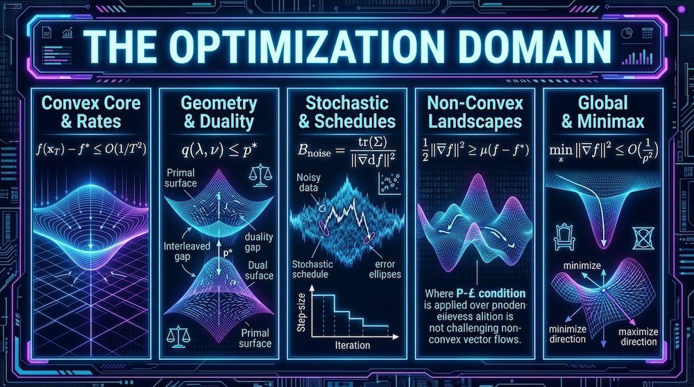
A standalone tutorial, not a survey: an optimization problem as a function and a set and a method as a sequence of oracle queries, what convexity buys and the one pathology it leaves, duality and KKT with the SVM's support vectors named by complementary slackness and the log-partition's conjugate as negative entropy, the rates of gradient descent, heavy ball and Nesterov against their theorems and against Nesterov's worst-case function, mirror descent and natural gradient as steepest descent under a different geometry, Adam as a diagonal preconditioner with the counter-example on which it fails and the block-heterogeneous quadratic on which it wins, Shampoo, SOAP and Muon as steepest descent under the spectral norm with the 2025–26 scoreboard quoted from the neutral benchmarks, the stochastic regime from the Robbins–Monro hand-off through the noise floor, the gradient noise scale, variance reduction, schedules on the noisy quadratic model, warmup and the equilibrium norm that weight decay actually sets, double descent with the bias–variance decomposition exact on the linear model and benign overfitting as the condition under which interpolating is harmless, what a stationary-point guarantee promises on a non-convex function and the lower bounds that say nothing more can be promised, saddles, Polyak–Łojasiewicz, the conservative-gradient theorem under autodiff on a ReLU net, benign landscapes, lazy versus feature learning, the edge of stability, implicit bias and the sharpness that is not a property of the function, deterministic global optimization from branch-and-bound through αBB and Lasserre to the ReLU verifiers where it is load-bearing today, Langevin, Bayesian optimization and quantization as the stochastic and discrete alternatives, minimax as not-descent, seventeen checkpoint exercises, a list of the common misreadings, and an appendix that grades every connection to our earlier posts by how much it actually proves.
Start with the one sentence everything else hangs on, stated with the three words that are usually dropped. An optimization problem is a function and a set; a method is a sequence of queries to an oracle about that function; a guarantee is a statement about the worst function in a class after a fixed number of queries. Nothing else is primitive. "Converges", "rate", "optimal", "condition number", "step size" and "stationary" are all defined in terms of those three objects, and every time one of them produces a paradox it is because the class or the oracle was left implicit and two readers filled it in differently. Say that gradient descent on a smooth convex function "converges at rate " and a reader who has the class convex, -smooth in mind is right; a reader who has strongly convex functions in mind is also right, and gets a geometric rate instead; and a reader who is thinking of a quadratic with a single bad direction and a particular start is right to observe that the first reader's bound is off by a factor of a thousand on it. §3 shows all three with numbers. Every result in this piece is a consequence of taking that sentence seriously, including the cases where a method that provably converges on every function in a class is the wrong method on the one function you have, and where a method with no guarantee at all is the one that trains your model.
Here is the claim, at the width the mathematics supports, because the tidy version is wrong in both directions. We are not claiming that training a neural network is convex optimization wearing a hat, and we are not claiming that a practitioner needs Nesterov's lower bound to pick a learning rate — nobody does, and we say exactly where the convex theory stops applying. The claim is this:
Optimization theory supplies the class in which each training claim is a theorem, and the rate at which it is one. "Gradient descent with step reaches an -stationary point of a smooth function in steps" is an exact theorem, convex or not, and nothing better is possible for a first-order method. "Momentum accelerates" is a theorem on the class of smooth strongly convex functions, with the exponent in place of , and a heuristic everywhere else. "Adam converges" is false as stated — there is a convex problem on which it does not — and true for the variant that monotonises its second moment. "A learning-rate cooldown drops the loss" is a one-line computation on a noisy quadratic. "SGD finds flat minima that generalise" is a hypothesis with a counter-example attached to the word "flat". "Deep networks have no bad local minima" is false as stated and true for matrix factorisation. The value of the lens is not that everything is secretly convex. It is that it tells you which of your claims are theorems, which are theorems on a class your loss is not in, and which are hypotheses.
Every connection in this piece carries one of four labels — the same four as our Information Domain and Probability Domain pieces, so the three can be read as chapters of one book. If you are here for the learning-rate questions, skip to §5 and come back to this table the first time a label stops you:
| Level | What it means | What you may conclude |
|---|---|---|
| L1 — exact theorem | The quantities and assumptions match a proven result | An identity or a bound that holds under the listed assumptions — not necessarily tight, and the assumptions need not hold in the application |
| L2 — variational correspondence | The objective has the same optimisation structure, with every term defined | A formal analogy you can compute with |
| L3 — engineering heuristic | A similar mechanism appears, with assumptions unchecked | Design intuition, to be validated |
| L4 — speculative analogy | A resemblance without a derivation | A hypothesis to test, nothing more |
Where a connection has two parts we grade both: the theorem, and the claim that the training problem satisfies its hypotheses. Nesterov's acceleration is L1; "a transformer's loss is smooth and strongly convex near the end of training, so momentum is accelerating it" is L3; the two grades sit side by side in §3 and §4 rather than being averaged into one. In this piece the second grade bites harder than it did in the earlier two, because almost every theorem below is stated for a class — convex, smooth, PL, strict-saddle — and the first question about any training loss is which class, if any, it is in.
Four running examples carry the same numbers through the whole piece, so that when two sections seem to disagree you can see which one is wrong.
- E1 — the quadratic with condition number : with eigenvalues log-spaced in . The step-size boundary at (§0), the rates of gradient descent, heavy ball and Nesterov against their theorems (§3), the block-heterogeneous version on which one learning rate fails and a diagonal preconditioner is exact (§4), the noise floor under additive gradient noise (§5), and the noisy quadratic model on which every learning-rate schedule can be computed exactly (§5).
- E2 — logistic regression, in two forms: a 30-dimensional problem on which the batch-size curve and the gradient noise scale are measured (§5), and our Probability Domain's two-class Gaussian mixture in with Bayes risk , on which the three errors of the excess risk — approximation, estimation, optimization — are separated (§5.7).
- E3 — rank- matrix sensing, : a non-convex problem that gradient descent solves from every random start (§0), the strict saddle at that it never leaves when started there (§0), the theorem that explains both (§7), and what over-parameterising the factor costs (§7).
- E4 — the two-dimensional Rastrigin function, on : the problem on which branch-and-bound certifies the global minimum and on which the number of boxes it needs grows exponentially with dimension (§8), on which local search succeeds one time in a hundred, annealed Langevin one time in nine and Bayesian optimization finds a better point than random search with the same budget (§8).
Prerequisites. Calculus, including the gradient and the Hessian; linear algebra at the level of eigenvalues and the singular value decomposition; the words "mean" and "variance"; having trained something with SGD or Adam. No convex analysis is assumed, and some is taught: §1 to §3 build the objects the rest of the piece is written in — the convex function, the subgradient, the conjugate, the oracle and the condition number — from those prerequisites, and build only those. Two kinds of section follow. §1 to §5 and §6.2–§6.4 are built from the stated prerequisites: each theorem they use is stated with its hypotheses and either proved, sketched, or reduced to a named result the text has already given. §4.6, §6.1, §7, §8.2 and §9 state theorems with their assumptions and a reference and do not pretend to prove them; those sections are read for what a theorem licenses and what it does not. If you know convex optimization, §1 to §3 are a fast re-read with the machine-learning consumers attached; the new material for you starts at §4.
Three reading paths, and the sections none of them may skip. The piece is six modules — Convex core §1–§3; Geometry §4; Stochastic §5; Non-convex §6–§7; Global §8; Minimax and the rest §9–§11 — and the paths are routes through them.
The fast path, for the practitioner who wants the learning-rate answers and will come back for the objects, has fourteen stops, each marked by a banner under its heading: §0, §1.4, §3.2, §3.3, §4.4, §4.5, §5.1, §5.2, §5.4, §5.6, §6.2, §7.3, §10 and §11, in that order. Its destination is §5.4, the schedule section, which is stop 9. If you only have two hours, start here and stop at §11. The fast path is a route through fourteen selected results, not a substitute for the objects behind their proofs: a claim quoted at a stop is proved in a section the path skips, and the hypotheses the stop's number rests on are stated there.
The full practitioner path is §0 → §1 → §3 → §4 → §5 → §6 → §7 → §10 → §11, doing the checkpoint exercises that lie on it. The theorist path is §0 → §1 → §2 → §3 → §4 → §5 → §6 → §7 → §8 → §9 → §10 → §11. §1, §3 and §5 are on both full paths: §1 is the object, §3 is what a rate is and why momentum is a theorem, and §5 is the regime every training loop actually runs in. §2 (duality) is the bridge to our Information Domain piece and the section a reader who liked that one should take. §8 (global optimization) is the section the board asked for by name and the one most likely to be new to a deep-learning reader; it is on the theorist path and recommended on the other, because the practitioner's intuition that "global" is the goal is corrected there. §9 (minimax) is the on-ramp to our game-theory pieces and can be read on its own. The history is Appendix A, the audit of where this machinery is load-bearing outside machine learning is Appendix B, two toy cases of ours are Appendix C, and the graded ledger of how this piece bears on our earlier posts is Appendix D. This piece stands alone: where an earlier post of ours is relevant it is linked as a citation, the way a paper would be, and nothing below requires having read it.
Six common misreadings, up front. The material below is misapplied in a few recurring ways; §10 gives the action that replaces each, and the section named proves the correction. (1) Reading a rate without its class: Nesterov's is a theorem on smooth convex functions and says nothing about a transformer's loss (§3.4, §6.2). (2) Reading "flat" as a property of the function: sharpness changes under reparametrisation, so every flatness claim needs a normalisation before it is well-defined (§7.5). (3) Reading "Adam converged" as a statement about the problem: at a constant step it is a statement about the noise floor, and without a schedule it is not a convergence claim at all (§5.1, §5.4, §6.2). (4) Reading a theorem on the simplex as a theorem in the logits: the KL-penalised objective is concave in the probabilities and not in the parameters, already for two actions (§1.5, §2.4, §9.2). (5) Reading the constants as transferable: accelerates nothing in the sense, is the boundary and not a safe step, and Adam's bounds a coordinate's step only up to a factor — for one gradient after a quiet stretch, over all gradient histories (§3.3, §0, §4.4). (6) Reading a certificate into a method that has none: restarts, annealing and Bayesian optimization report a success rate, branch-and-bound reports a proof, and only the latter is "global" (§8.1, §8.3).
Companion code. Every number in a code block below is copied from the printed output of
worked_numbers.py, a single NumPy script with 53 numbered sections, float64, CPU-only, that ships with this piece; a section number in the form§Nbeside a block names the section that printed it, the numbers are verbatim, and where a line's label has been shortened for the page the full label is in the script's output file. The script's generator is seeded once,default_rng(20261105), and the sections draw from it in order, so that a reader running the script reproduces every line, line for line, in the pinned environment (requirements.txt: Python 3.14.5, NumPy 2.5.3). On another Python or NumPy build the closed-form lines are identical and the seeded Monte Carlo lines agree within their printed standard errors but not necessarily to the digit — a different build can round, and therefore iterate, differently — so the check elsewhere is agreement within tolerance, not identical digits (an independent re-run on Linux, Python 3.13 / NumPy 2.3, reproduced forty of forty-nine sections exactly and moved nine within their tolerances, with every section's reading surviving); every Monte Carlo value that is compared to a theory value is printed with its standard error, computed from the draws the section already makes. The script takes about eleven minutes on a laptop; the bulk of that is the batch-size sweep of§17and the branch-and-bound of§32, both of which are the point. Atest_worked_numbers.pybeside the script re-derives the closed-form values the blocks are compared against. The two companion notebooks —00_convex_machinery.ipynb(the puzzles, convexity, duality, rates, mirror descent and natural gradient, Adam's counter-example, the orthogonalised update, the stochastic regime and schedules, the three errors, and the critic-round counter-examples: the heavy-ball prefactor, KL in the logits, Adam's step after a quiet stretch and over all histories, and AdamW against the exact prox) and01_nonconvex_and_global.ipynb(stationarity, saddles, PL, autodiff at a kink, benign landscapes, lazy versus feature learning, the edge of stability, implicit bias, mode connectivity, branch-and-bound, Langevin, Bayesian optimization, verification, quantisation, minimax, compressed sensing, double descent, the stable-ReLU interval counter-example, the GRPO baseline, the Goemans–Williamson triangle, the Euler–Langevin variance and the two saddle-method spectral radii) — ship beside it, built from those sections cell by cell; each cell restores the script's generator state at its section, so a notebook prints this piece's numbers whether it is run top to bottom or one cell at a time. A reader on the fast path who runs only the cells its stops quote —§1,§2,§3,§7,§12,§13,§14,§15,§16,§17,§19,§20,§21,§22,§28,§42,§46and§48, eighteen cells — sees every number the fast path quotes, for the same reason: each of those cells was run on its own in a fresh interpreter after the setup cell, and none reads a variable that an earlier cell defines (the setup cell holds every helper, and the state each cell needs beyond the generator is computed inside it).
Units and conventions, once. is the function to be minimised; its infimum; a minimiser when one exists. is the Lipschitz constant of the gradient (" is -smooth"), the strong-convexity constant, the condition number. and are both step sizes — when the step is a design choice, when it is the subject of a theorem — because the two literatures use different letters and we quote both. is the number of steps, the current one. with no subscript is Euclidean; on a matrix is the spectral norm, the Frobenius norm, the nuclear norm. Logarithms are natural. "a.s." means almost surely. A rate is an upper bound on or on as a function of , over a class; a lower bound is a statement that no method in a class of methods can do better on the worst function in a class of functions.
0. Three puzzles that are one puzzle
Fast path · stop 1 of 14. Next stop: §1.4. This section's numbers run in
00_convex_machinery.ipynb.
Optimization is counter-intuitive in a specific way. The puzzles that trip people up are almost never about the arithmetic of a step; they are about which class the function is in and which oracle the method is talking to. Three of them, each resolved by naming the object the question left out, and each the seed of a section below.
Puzzle 1 — one step size, two verdicts. Take E1 at : twenty eigenvalues log-spaced from to , so . Run gradient descent with the step written as a multiple of , for 200 steps from the all-ones vector:
§1 Puzzle 1: one step size, two verdicts — GD on a quadratic at eta = 0.5/L, 1.9/L, 2.1/L
eta = 0.50/L f(x_200) = 1.7290e-01 contraction factor max|1-eta*lambda| = 0.9950
eta = 1.00/L f(x_200) = 1.4182e-02 contraction factor max|1-eta*lambda| = 0.9900
eta = 1.90/L f(x_200) = 2.7082e-04 contraction factor max|1-eta*lambda| = 0.9810
eta = 1.99/L f(x_200) = 8.9771e-01 contraction factor max|1-eta*lambda| = 0.9900
eta = 2.01/L f(x_200) = 2.6762e+03 contraction factor max|1-eta*lambda| = 1.0100
eta = 2.10/L f(x_200) = 1.8032e+18 contraction factor max|1-eta*lambda| = 1.1000
L = 100.0, mu = 1.0, kappa = 100; the boundary is eta = 2/L = 0.0200Every step below converges, and the best of the six is — fifty times better than the "safe" after the same 200 steps — not because a larger step is always better but because the quantity that decides, , is smallest when the two ends of the spectrum contract equally: at the stiffest direction contracts at per step and the softest at ; at the stiffest direction oscillates at and the run is worse than at , though still convergent. (The optimum is , where the two factors coincide.) Every step above diverges, and the divergence is not gradual: at the loss after 200 steps is , at it is . The contraction factor of the worst eigen-direction is a function of the step and the largest curvature only. Now the puzzle. The step that trains a transformer under Adam is or so, and a practitioner who has never seen a loss diverge at that step takes it to a convex logistic regression and watches it oscillate. The resolution is the oracle, not the function: Adam's update is not the gradient, it is the gradient divided coordinate-wise by a running root-mean-square of itself, so its step has the units of the parameter and not of the parameter divided by curvature, and the rule does not apply to it in the form above (it applies in another form: §4.4). The same number is a step size for one method and a trust-region radius for the other. §1.4 names and , §3 turns the contraction factor into a rate, and §7.3 shows a network whose top curvature is driven to exactly by the training dynamics and held there.
Puzzle 2 — the same loss, zero training error twice, two different models. Take a least-squares problem with parameters and examples, generated by a sparse truth (ten nonzero coefficients). Any method that reaches zero training loss has solved the problem as posed. Run two from the origin — plain gradient descent, and sign descent, which is Adam with both moving averages switched off — and compare them with the minimum-norm interpolant that the pseudo-inverse computes:
§2 Puzzle 2: same loss, zero training error twice, two different models (d > n least squares)
GD from 0 train MSE = 9.15e-32 test MSE = 54.7481 ||w||_2 = 3.336 ||w||_1 = 36.74 ||w||_inf = 0.933
sign descent from 0 train MSE = 8.58e-05 test MSE = 68.2429 ||w||_2 = 3.867 ||w||_1 = 50.48 ||w||_inf = 0.348
min-norm (pinv) train MSE = 4.27e-28 test MSE = 54.7481 ||w||_2 = 3.336 ||w||_1 = 36.74 ||w||_inf = 0.933
||w_GD - w_minnorm||_2 = 9.95e-15 (GD from zero converges to the min-norm interpolant)Both optimizers minimised the same function to (essentially) the same value. They returned different vectors, with different test errors, and gradient descent's vector is the minimum-Euclidean-norm interpolant to fourteen digits while sign descent's is a different interpolant with a smaller norm and a larger norm. The loss did not choose the model; the method did, by a bias the loss never mentions. This is a theorem for gradient descent on least squares (the iterates never leave the row space of , so the limit is the min-norm solution — a four-line argument, §7.4) and a theorem of a different kind for sign descent (§7.4 states it with its grade). The practical content: when a problem has many global minima — every over-parameterised problem does — "which optimizer" is a question about which minimum, not about speed, and the two optimizers that reach zero loss fastest need not reach the same place. §4 and §7.4 carry this through to the implicit bias of Adam versus SGD on real networks, with the grade the evidence supports.
Puzzle 3 — a non-convex problem that gradient descent solves from any random start. E3 at rank one: , Gaussian sensing matrices, and , which is a quartic in and not convex (it has two global minima, , and a convex function has a convex set of minimisers). Run gradient descent from a hundred random starts, and once from the origin:
§3 Puzzle 3: a non-convex problem that gradient descent solves from any random start (rank-1 matrix sensing)
100 random starts (scale 0.1), step 0.1: reached a global minimiser (x = +/-u to 1e-4) in 100/100 runs; steps to f < 1e-12: median 84, max 108
Hessian at the saddle x = 0: lambda_min = -2.5073, lambda_max = 0.5781 (lambda_min < 0: x = 0 is a strict saddle, not a minimum)
started exactly at x = 0: f after 20000 steps = 6.1520e-01 (gradient descent never leaves a stationary point)A hundred of a hundred, in about ninety steps, on a function that no convexity theorem covers; and a run that never moves, from a point where the gradient is exactly zero and the Hessian has a negative eigenvalue of — a strict saddle, from which the slightest push would have escaped in a few dozen steps (§6.3 measures how many). The resolution is the class: this function is not convex, but every one of its local minima is global and every one of its saddles is strict (§7.1 states the theorem with the sample-size condition that makes it true), and on that class gradient descent from a random start converges to a global minimum with probability one (§6.3). "Non-convex" is not one class; it is everything that is not convex, and the first job of §6–§8 is to separate the non-convex problems that have a theorem from the ones that have only hardness results — and to say, honestly, which of those a neural network is.
All three puzzles are the same puzzle: a method was described by what it does on one class of problems, and used on another. The rest of this piece is the catalogue of classes.
1. What convexity buys, and the one pathology it leaves
1.1 The definition is a statement about chords
A set is convex if the segment between any two of its points lies in it: for every . A function on a convex set is convex if it lies below its chords,
strictly convex if the inequality is strict for and , and concave if is convex. That is the whole definition; everything else in this section is a consequence of it, and the first thing to notice is what it does not mention: derivatives. Convexity is a property of the graph, and a function can be convex without being differentiable anywhere a step wants to go (, the hinge loss, the penalty). The definition is also checkable, which Jensen's inequality (our Probability Domain's §3.5) turns into a test: draw chords at random and count the violations.
§4 Convexity is checked on chords: Jensen on three functions, 10,000 random chords each
x^2 fraction of chords with f(theta a+(1-theta) b) > theta f(a)+(1-theta) f(b): 0.0000
exp(x) fraction of chords with f(theta a+(1-theta) b) > theta f(a)+(1-theta) f(b): 0.0000
log-sum-exp(x, 0) fraction of chords with f(theta a+(1-theta) b) > theta f(a)+(1-theta) f(b): 0.0000
sin(x) fraction of chords with f(theta a+(1-theta) b) > theta f(a)+(1-theta) f(b): 0.5034
sqrt|x| fraction of chords with f(theta a+(1-theta) b) > theta f(a)+(1-theta) f(b): 0.5586The third row is the one to keep: is the logistic loss of a single example as a function of its logit, and it is convex — which is why logistic regression, a linear logit followed by that loss, is a convex problem in its weights. (A convex function of an affine function is convex; a sum of convex functions is convex; a non-negative multiple is convex. Those three closure rules, plus "pointwise maximum of convex functions is convex", are the calculus with which one certifies a loss. Boyd & Vandenberghe's chapter 3 is the reference and is free.) The last two rows are the shape of the trouble ahead: is convex on half its domain and concave on the other, and is a cusp that is concave on each side — the shape of an penalty with , which is exactly the sparsity penalty whose minimisation is NP-hard (§8.5).
1.2 First-order conditions, and the subgradient
For differentiable on an open convex set, convexity is equivalent to the first-order condition
the tangent plane at lies below the graph everywhere; and for twice-differentiable to everywhere. The first-order condition is the one that does work, because it is a global statement obtained from a local computation: one gradient at bounds from below on the whole domain. That is the mechanism under every convergence proof in §3.
When is convex but not differentiable at , the tangent plane is replaced by the set of all planes that lie below the graph and touch it at : the subdifferential
a closed convex set, non-empty at every interior point of the domain for a convex (Rockafellar's Theorem 23.4), equal to where is differentiable. For it is away from zero and the whole interval at zero. For the hinge loss it is a segment at the kink. A method that uses "a subgradient" at a kink has a choice to make there, and the §3.5 rates for the subgradient method are rates for any choice.
1.3 Local is global: the proof, in four lines
Theorem. If is convex and is a local minimiser, it is a global minimiser; the set of global minimisers is convex; if is strictly convex it has at most one.
Proof. Suppose for some . For , . As the point enters every neighbourhood of with a smaller value, contradicting local minimality. Convexity of the minimiser set is the chord inequality applied to two minimisers; uniqueness under strict convexity is the same chord with a strict inequality.
The corollary that matters for a method: for a convex differentiable , if and only if is a global minimiser (one direction is the first-order condition with ; the other is calculus), and for a nondifferentiable one, if and only if is a global minimiser. A stationary point is the answer. Every "stationary point" guarantee of §6 is this corollary with the convexity hypothesis removed, and §6.2 is about what is left of it when it is.
1.4 Smoothness, strong convexity, and the one number to know
Fast path · stop 2 of 14. Next stop: §3.2.
Two quantitative strengthenings of convexity give the two numbers that every rate in this piece is written in.
is -smooth if its gradient is -Lipschitz, ; for twice-differentiable this is — both sides, since the gradient of has Lipschitz constant although its Hessian, , is below . The one-sided is the weaker upper-curvature condition; it is all the descent lemma below uses, and it coincides with smoothness exactly when is convex, because convexity supplies the other side. The distinction matters from §6 on, where smoothness is used without convexity: there the two-sided condition is the hypothesis, and a function whose curvature is bounded above but not below has a descent lemma and no . Its consequence is the descent lemma, an upper quadratic:
(Proof: , subtract , bound the integrand by with the Lipschitz property, integrate.) Put and the lemma says : a gradient step of size decreases by a definite amount, with the largest guaranteed decrease at . The descent lemma needs no convexity and only the upper side of the Hessian bound, which is why it survives into §6 — and it is why Puzzle 1's boundary was : on a quadratic the lemma is exact, the contraction factor of each eigen-direction is , and the direction with crosses from contraction to expansion at exactly .
is -strongly convex if is convex, equivalently — a lower quadratic — equivalently . Its consequences: a unique minimiser; (minimise the lower quadratic over ), so that a small gradient certifies a small suboptimality — the inequality that §6.4 generalises beyond convexity as Polyak–Łojasiewicz; and .
The condition number is the ratio of the two, and it is the one number a practitioner should be able to estimate for their problem, because it governs every rate in §3: gradient descent needs steps, momentum , and nothing first-order does better. On a quadratic it is the ratio of extreme Hessian eigenvalues; on a least-squares problem it is the squared ratio of extreme singular values of the design matrix; on a logistic regression it is bounded by the same ratio times a factor from the curvature of the loss. On a deep network it is undefined in the strongly convex sense ( at best, negative curvature in general) and the useful analogues are the ones §7 introduces: the top Hessian eigenvalue, which plays (§7.3), and the smallest eigenvalue of the tangent kernel on the data, which plays (§7.2).
The practitioner's reading. A learning rate is a fraction of and you do not know ; everything in a training loop that touches the learning rate is a way of estimating or evading it. A warmup estimates it by starting small (§5.5). Adam evades it by normalising per coordinate (§4.4). Gradient clipping bounds the step where is locally large (§5.2). Line search measures it directly and is not used in deep learning because each measurement costs a forward pass on a stochastic objective. And the edge-of-stability phenomenon of §7.3 is the one behaviour none of the convex theory anticipates: on a network under gradient descent the top curvature rises along the trajectory until it meets and is held there by a feedback in the dynamics — not an intention — so that ends up set by the step rather than the step by .
1.5 Where this touches a loss function already
- Least squares, ridge, logistic regression, softmax regression, SVM, lasso: convex in their weights. For each, a stationary point is the global optimum, the duality of §2 applies, and the rates of §3 are theorems about the training loop. The KL-penalised policy objective of RLHF (§2.4) is concave in the policy's probabilities on the simplex, and not in its logits — already for two actions, with no network in sight. Take zero reward, a uniform reference and : the objective is , and its second derivative changes sign once the policy is confident:
§43 The KL-penalised objective is concave in the policy's probabilities and NOT in its logits: a two-action counter-example
z J(z) = -KL(Ber(sigmoid z) || Ber(1/2)) J''(z) closed form J''(z) by central differences (h = 1e-4)
0.0 -0.000000 -0.25000 -0.25000
1.0 -0.110944 -0.10575 -0.10575
1.5 -0.218096 -0.00705 -0.00705
2.0 -0.327813 +0.05493 +0.05493
3.0 -0.502282 +0.07750 +0.07750: the sigmoid's own curvature overwhelms the KL's, the function is not concave in , and a theorem proved over the simplex (§2.4's closed form) says nothing about the landscape a gradient method sees in the logits — let alone in the weights of a network that produces them. This is the first instance of the rule the whole piece runs on: the class is a property of the parametrisation, not of the problem. When one of these is the problem — a linear probe, a calibration head, a reward model's last layer — the question "did it converge" has a yes/no answer, and the §3 rates say how many steps a yes costs.
- Any network with a hidden layer: not convex, and not for a subtle reason. Permuting the hidden units of a trained network gives another network with the same function and the same loss; the midpoint of the two parameter vectors is, in general, a different function with a higher loss (§7.6 measures the barrier: zero between two runs from one initialisation, a midpoint loss five times the endpoints' between runs from two). A convex function's minimisers form a convex set; these do not. Beyond symmetry, Blum & Rivest (1992) show that deciding whether a three-node network can fit a dataset is NP-complete, so no polynomial algorithm minimises the training loss of every network on every dataset unless P = NP. Both facts are L1, and neither says anything about the typical instance, which is §7's subject.
- The parametrisation can be chosen for convexity. A one-hidden-layer network is non-convex in its weights but convex in the measure over hidden units (Bengio et al. 2006; Bach 2017) — which is the mean-field view of §7.2 and the reason global convergence theorems exist in the infinite-width limit. Phase retrieval is non-convex in and convex (a semidefinite program) in ; matrix completion is non-convex in the factors and convex in the matrix with a nuclear-norm penalty. In each case the convex formulation is the one with a theorem and the non-convex one is the one that runs, and §7.1 is about when the non-convex one inherits the theorem.
- A loss can be convex and still have in practice. Logistic regression on linearly separable data has no minimiser — the loss tends to zero as along any separating direction — and gradient descent runs forever, which is not a failure but the setting of §7.4, where which direction it runs along is a theorem.
Checkpoint exercise 1. The cross-entropy loss is convex in the logits . Show it (hint: it equals , and log-sum-exp is convex by the Hessian test or the §4 chord test). Then show that it stays convex in the weights of the layer that produces when the features are fixed — the logits are affine in , and a convex function of an affine map is convex — which is why a linear probe on frozen features is a convex problem with a unique minimum value. Finally explain why that convexity is lost once the layers that produce are trained jointly with , using the permutation argument: permuting the hidden units gives a second minimiser, and the midpoint of the two is not one. The two facts together are the difference between fitting a probe and fine-tuning end to end. Exercise 2. For E1 with , compute at and at and check that both equal — the first from the softest direction (), the second from the stiffest (). Then explain why the row of §1 is nevertheless sixty-three times worse than the row after 200 steps, although the surviving amplitude decays at the same rate in both: weights that amplitude by its curvature, and the two surviving directions differ in curvature by (§47 prints the two shares, against ). The moral is the one §0 drew: a step just below the stability boundary is not a fast step, because the direction it leaves oscillating is the one the loss weights most.
2. Duality, KKT, and the conjugate
This section is on the theorist path and is the bridge to our Information Domain piece. A practitioner may read §2.3 for the support vectors and §2.4 for the one closed form that RLHF and DPO are built on, and skip the rest on a first pass.
2.1 The Lagrangian and weak duality
The constrained problem is subject to , , and , , over a domain . Its Lagrangian attaches a price to each constraint:
and the dual function is concave in whatever and are — it is an infimum of affine functions of the multipliers. Weak duality: for every and , because for any feasible , (the penalty terms are ). So the dual problem is a convex problem whose value is a lower bound on the primal, for any primal, convex or not. The gap is the duality gap.
Weak duality is what a lower bound is, operationally: §8.1's branch-and-bound certifies a global minimum by producing a lower bound that meets the best value found, and a Lagrangian relaxation is one of the standard ways to produce one. The gap can be enormous. For the primal value is , but is unbounded below in for every multiplier, so and : the dual certifies nothing. Concave objectives over a box are the elementary hard case of global optimization (§8.1), and their dual gap is the elementary reason.
2.2 Strong duality, Slater, and when the gap closes
Strong duality is . It holds for convex problems under a constraint qualification; the standard one is Slater's condition: convex, affine, and some strictly feasible point exists ( for the non-affine ). Under it the dual optimum is attained; and when a primal optimiser exists as well — Slater gives and dual attainment, not primal attainment, for which one adds a compact feasible set or a coercive — the primal–dual pair is a saddle point of the Lagrangian: minimises and maximises — the minimax structure of §9 in its convex–concave, always-solvable form. Strong duality also holds for every linear program with a finite value, with no Slater (LP duality, 1947 — Appendix A); it can fail for convex problems without Slater (the standard example is s.t. , : , ).
Here it is on a problem a practitioner has run. The bias-free soft-margin SVM has the dual with , and . Run projected gradient ascent on the dual and evaluate both objectives along the way:
§5 Weak and strong duality on a bias-free soft-margin SVM: primal and dual objectives meet; KKT names the support vectors
iter 1: dual = 0.628651 primal(w(a)) = 30.334389 gap = 2.97e+01
iter 10: dual = 2.875073 primal(w(a)) = 19.140024 gap = 1.63e+01
iter 100: dual = 12.766033 primal(w(a)) = 13.587708 gap = 8.22e-01
iter 1000: dual = 13.408400 primal(w(a)) = 13.420371 gap = 1.20e-02
iter 20000: dual = 13.412993 primal(w(a)) = 13.412993 gap = 3.55e-15
support vectors (alpha > 1e-6): 17/60; alpha = C (inside margin or misclassified): 15; 0 < alpha < C (exactly on the margin, y w.x = 1): 2
max |y w.x - 1| over the on-margin set = 3.89e-15; min y w.x over alpha = 0 points = 1.0389 (>= 1: complementary slackness)At every iteration the dual value is below the primal value (weak duality), the two meet at the optimum to machine precision (strong duality: the problem is a convex quadratic with affine constraints), and — the useful part — the gap is a stopping criterion you can compute: at iteration 1000 the solution is certified to within of optimal without knowing the optimum. Every interior-point solver (§3.6) reports exactly this number.
2.3 KKT, and complementary slackness names the support vectors
At a primal–dual optimum of a convex problem with strong duality and differentiable functions, the Karush–Kuhn–Tucker conditions hold:
- primal feasibility , ;
- dual feasibility ;
- stationarity ;
- complementary slackness for every .
For a convex problem these are also sufficient. Condition 4 is the one with content: a constraint either binds () or its price is zero (). On the SVM the constraints are the margins, and the block above reads them off: 43 of the 60 points have and sit strictly outside the margin (their smallest margin is ); 15 have and are inside it or misclassified; and exactly two have and sit exactly on the margin, to fifteen digits. The decision boundary is determined by seventeen points — the support vectors — and the other 43 could be deleted without changing it. That is not a heuristic about SVMs; it is KKT condition 4 read as a statement about the data.
For a non-convex problem the KKT conditions are necessary at a local optimum under a constraint qualification (the Lagrange multiplier theorem) and not sufficient; a KKT point can be a saddle or a local maximum. §6 is the unconstrained version of that sentence.
2.4 The Fenchel conjugate: log-partition ↔ negative entropy, and the one closed form under RLHF
The Fenchel conjugate of is : the largest gap between a linear function with slope and . It is convex always (a sup of affine functions), and for convex closed , (Fenchel–Moreau). The conjugate is the engine under Lagrangian duality — the dual function of a linearly constrained problem is a conjugate in disguise — and under the two identities that tie this piece to our Information Domain one.
Identity 1 (log-sum-exp ↔ negative entropy). On the simplex , the conjugate of the negative entropy is the log-partition function: , with the sup attained at . Equivalently . That is the variational characterisation of the softmax our Information Domain's §9.8 stated; here it is a conjugate pair, which means it comes with a method: maximise over the simplex by mirror descent (§4.2) and watch it find the softmax.
§6 Fenchel conjugate of log-sum-exp is negative entropy; the KL-penalised objective has a Gibbs closed form (W41 bridge)
A(theta) = log sum exp(theta) = 2.440190; max_p <theta,p> + H(p) by exponentiated gradient = 2.440190; argmax p = [0.2369 0.0871 0.0321 0.6439]; softmax(theta) = [0.2369 0.0871 0.0321 0.6439]
KL-penalised argmax by EG = [0.866 0.0762 0.006 0.0519]; closed form pi exp(r/beta)/Z = [0.866 0.0762 0.006 0.0519]; optimal value 1.459336 vs beta log Z = 1.459336Identity 2 (the KL-penalised maximisation has a Gibbs solution). For a reference distribution , reward and temperature ,
which is Identity 1 with the entropy replaced by a relative entropy, i.e. the conjugate of . The second line of §6 checks both the maximiser and the value. This is the closed form on which the RLHF objective of our Information Domain §10.3 rests, and the step on which DPO (Rafailov et al. 2023) is built: substituting into the Bradley–Terry preference likelihood eliminates the reward model. Grade: the identity is L1 and holds per prompt in the tabular case, over the simplex; "a policy network trained by gradient ascent on the penalised objective reaches " is a statement about a non-convex problem — non-convex already in the logits of a two-action tabular policy, §1.5's §43, before any network — and is L3; and the identity says nothing about the estimation of , which is where the practical difficulty sits. The conjugate structure also gives the mirror-descent view of the KL-penalised updates (PPO's penalty form, the objective GRPO carries): a KL-penalised step is a proximal step in the Bregman geometry of §4.2, which is why its closed form is multiplicative. PPO's clipped form is a different object, §9.2.
Identity 3 (Fisher is the Hessian of KL). , the Fisher information. This is the identity under natural gradient, and §4.3 checks it numerically in two parametrisations and uses it.
Checkpoint exercise 3. Derive the SVM dual of §2.2 from the Lagrangian: introduce slacks , , write , minimise over and in closed form, and show the box constraint is what is left. Exercise 4. Show that at puts all mass on and at returns , and compute the KL between and as a function of on the four-state example of §6.
3. Rates and lower bounds: what a guarantee is
3.1 The oracle model, and what "optimal" means for a method
Nemirovski & Yudin (1983) made the question precise. A first-order oracle returns and (or a subgradient) at a query point; a method is any rule that chooses the next query from the answers so far; the complexity of a class of functions is the smallest number of queries that guarantees for every . A rate is an upper bound on that number achieved by a particular method; a lower bound is a proof that no method does better on the worst function in the class. A method is optimal for a class when its rate matches the class's lower bound up to constants.
Three things follow from the definition that are routinely forgotten. A rate is a worst-case statement: the function you have may be far from the worst in its class, and gradient descent on it may beat its bound by a large factor (§7 below shows a factor of for a reason that is a one-line computation). A lower bound is a statement about a function in the class, constructed to defeat every method; it says nothing about yours. And a class is a choice: the same method has a different rate on convex, -smooth, on -strongly convex, -smooth, and on -smooth with no convexity, and the three are , and " for ", which are not comparable because they bound different quantities.
3.2 Gradient descent: the two convex rates, and the condition number as the exponent
Fast path · stop 3 of 14. Next stop: §3.3.
Theorem (smooth convex). If is convex and -smooth, gradient descent with satisfies .
Sketch. The descent lemma gives ; the first-order condition at against gives ; combining the two with the identity shows that is non-increasing and that ; since is non-increasing, the last term is at most the average. (Bubeck 2015, Thm 3.3; Nesterov 2018, Thm 2.1.14.)
Theorem (smooth strongly convex). If in addition is -strongly convex, gradient descent with satisfies and ; with the factor improves to on the distance.
Sketch. Strong convexity and smoothness together give (Nesterov's Thm 2.1.12); expand and apply it. On a quadratic every direction contracts by per step, and : the bound is the worst direction's contraction, and , being quadratic in the distance, contracts by its square.
So the number of steps to reach accuracy is : the condition number is the exponent's denominator, and doubling doubles the steps. Here are the two theorems on E1, with heavy ball and Nesterov's method beside them for §3.3:
§7 Rates on a quadratic: GD, heavy ball and Nesterov at kappa = 10, 100, 1000, 10,000 — iterations to f - f* < 1e-8, against the theorems' upper bounds
kappa GD iters GD bound (1-1/kappa)^2t HB iters Nesterov iters NAG bound (1-1/sqrt kappa)^t
10 69 91 18 25 52
100 703 1036 71 88 204
1000 6976 11370 263 291 730
10000 69417 123943 953 935 2536
(a bound is an upper bound: the worst direction holds only 1/d of the initial energy here, so GD beats its bound by a factor ~1.5)Read the first three columns against the theorem. Gradient descent's iterations grow by a factor of ten per decade of — linear in , as the exponent says — and the bound is above the measurement at every row by a factor between and . The factor is not slack in the theorem; it is the start. The bound assumes all of can sit in the slowest direction, and E1's start spreads it evenly over fifty directions, so the slowest one begins with a fiftieth of the energy and needs fewer steps. A reader who estimates for their problem and finds the bound pessimistic by a constant has found the constant; a reader who finds it pessimistic by a power of has the wrong class.
3.3 Momentum is a theorem: heavy ball and Nesterov, for
Fast path · stop 4 of 14. Next stop: §4.4.
Two methods add a memory of the previous step:
- Heavy ball (Polyak 1964): .
- Nesterov's accelerated gradient (1983): , — the gradient is evaluated at the extrapolated point.
Theorem (heavy ball on a quadratic). With and , , heavy ball on a strongly convex quadratic, started with zero momentum, satisfies ; equivalently, for every there is a with . The condition number enters as its square root. (Polyak 1964; the proof is the spectral radius of the companion matrix of each eigen-direction, which is at those constants.) The prefactor is not a constant, and the form the theorem is usually quoted in — a -independent in front of — is false: at the two extreme eigenvalues the companion matrix has a double root, so the iterate along those directions is , with the factor in front of growing linearly:
§42 Heavy ball's rate has a prefactor that grows with T: at the extreme eigenvalues the companion matrix has a double root, so x_T = (1 + c T) q^T x_0, not C q^T x_0
kappa = 100: alpha = 0.03306, beta = q^2 = 0.66942, q = 0.81818; double root +q at lam = mu, -q at lam = L; x_{-1} = x_0
T |x_T|/|x_0| at lam = mu (1 + (1-q) T) q^T at lam = L (1 + (1+q) T) q^T max over 2001 lam in [mu, L] q^T alone
10 3.7885e-01 3.7885e-01 2.5786e+00 2.5786e+00 2.5786e+00 1.3443e-01
100 3.6972e-08 3.6972e-08 3.5237e-07 3.5237e-07 3.5237e-07 1.9274e-09
1000 1.2937e-85 1.2937e-85 1.2874e-84 1.2874e-84 1.2874e-84 7.0766e-88At the stiff direction's iterate is times , the soft direction's times, and at the stiff direction is at times its start — momentum at these constants overshoots before it contracts. None of this touches the complexity: still holds at , because the logarithm of a polynomial is absorbed by the logarithm of ; it touches the statement, and a statement is what a theorem is. On non-quadratic strongly convex functions heavy ball with these constants can fail to converge — Lessard, Recht & Packard (2016) give a one-dimensional counter-example — so its rate is an L1 statement about quadratics and an L3 one about everything else.
Theorem (Nesterov, smooth convex). With and the momentum sequence , , (Nesterov 2018 Thm 2.2.2 gives ; the constant depends on the variant). (Nesterov, strongly convex.) With and constant , . Both hold for every smooth (strongly) convex function, not only quadratics — that is the difference from heavy ball, and the reason the extrapolated gradient is not a cosmetic change. The proofs go through an estimate sequence (Nesterov 2018 §2.2.1) or, more transparently, a potential function that is shown non-increasing (Bansal & Gupta 2019 give the four-line version).
The last three columns of §7 are the theorem on E1. Heavy ball and Nesterov's method grow by a factor of about per decade of , against gradient descent's ; at they need and steps against . The Nesterov bound is again above the measurement by a constant ( to ), for the same reason as before plus the factor.
The practitioner's reading of "momentum". Momentum in a training loop is heavy ball (, a learning rate), applied to a stochastic, non-convex objective. The theorem above says: on a strongly convex quadratic, with the right and tied to , it is faster. It does not say that accelerates anything — the acceleration constants are , which is at — and in the stochastic regime of §5 the role of is different: with gradient noise, momentum at a fixed effective step mainly averages the noise over steps and does not change the noise floor (§5.1; Kidambi et al. 2018 show heavy ball cannot beat plain SGD's rate in the stochastic least-squares setting). So the grade of "momentum helps my transformer": L1 on the quadratic model of its local curvature, L3 as a statement about the run. What is L1 without qualification is that the heavy-ball update's effective learning rate at a constant gradient is — ten times at — which is the first thing to remember when comparing learning rates across optimizers.
3.4 Nesterov's lower bound: no first-order method beats
The acceleration is not a trick that could be improved on by a cleverer method; it is optimal, and the proof is a single function.
Theorem (Nesterov 2018, Thm 2.1.7). For every with there is an -smooth convex function on such that any first-order method whose iterates lie in satisfies
The function is the chain , a tridiagonal quadratic whose gradient at a vector supported on the first coordinates is supported on the first : starting from , after gradient queries the method has only seen coordinates of a -dimensional problem whose solution lives on all of them, and the suboptimality of the best point on the first coordinates is the bound. The dimension grows with — the theorem is about a family of functions, one for each horizon — and that is the right way to run it:
§8 Nesterov's worst-case function f_{2t+1}: no first-order method beats 3 L ||x0 - x*||^2 / (32 (t+1)^2) at step t, and Nesterov's method is within a constant of it
t d=2t+1 GD gap f(x_t)-f* NAG gap lower bound 3LR^2/(32(t+1)^2) GD/bound NAG/bound NAG upper bound 4LR^2/(t+2)^2
1 3 0.046875 0.046875 0.020508 2.29 2.29 0.388889
2 5 0.040690 0.057292 0.015914 2.56 3.60 0.381944
5 11 0.031630 0.031762 0.009151 3.46 3.47 0.286848
10 21 0.024915 0.017577 0.005300 4.70 3.32 0.190025
20 41 0.018985 0.009321 0.002871 6.61 3.25 0.111603
50 101 0.012792 0.003915 0.001208 10.59 3.24 0.049559
100 201 0.009324 0.002003 0.000614 15.18 3.26 0.025696
(the function depends on t: at step t the method has only touched coordinates 1..t of a 2t+1-dimensional chain, whatever it did)Both methods are above the lower bound at every , as they must be. Nesterov's method sits at a constant the bound from onward — it is optimal up to that constant — while gradient descent's ratio grows like , which is exactly against . The right-hand column is the method's own upper bound, which it satisfies with room. Three things the table says that the theorem's statement does not: the lower bound is attained up to a constant, so there is no better first-order method to look for on this class; the gap between gradient descent and the optimum is a factor of , which at the steps of a training run would be enormous if the class applied; and the class does not apply to training a network — the lower bound is for the worst smooth convex function, and §6.2 gives the non-convex analogue, where the optimal rate is a different quantity altogether.
3.5 Nonsmooth: subgradient , proximal , FISTA
Remove smoothness and keep convexity. The subgradient method , , with the horizon-aware constant step ( a bound on , on the subgradients) satisfies (Bubeck 2015, Thm 3.2). With the decreasing step , which needs no horizon, the same bound holds for the best iterate up to a factor — is — and the log is removed by reporting the average of the last half of the iterates or a -weighted average: the rate is a property of the pair (schedule, iterate reported), not of the method alone, a distinction §5.4 returns to for SGD. The rate is optimal for the class of -Lipschitz convex functions — Nemirovski & Yudin's second lower bound. It is also not a descent method: a subgradient step can increase , which is why the guarantee is on the best iterate. Each halving of the error costs four times the steps.
But most nonsmooth losses in machine learning are structured: with smooth and simple — for the lasso, an indicator for a constraint set, the nuclear norm for low rank. The proximal gradient method , with , handles exactly at each step (for the prox is soft-thresholding; for an indicator it is projection; for the nuclear norm it is singular-value soft-thresholding) and recovers the smooth rates: at , and with Nesterov's extrapolation, which is FISTA (Beck & Teboulle 2009). Here are the three on a lasso with , , a five-sparse truth:
§9 Nonsmooth: subgradient O(1/sqrt t) vs proximal gradient O(1/t) vs FISTA O(1/t^2) on a lasso problem
t = 10: subgradient (best) 1.031e-01 proximal 1.364e-02 FISTA 1.410e-03
t = 100: subgradient (best) 9.048e-03 proximal 0.000e+00 FISTA 0.000e+00
t = 1000: subgradient (best) 2.548e-03 proximal 0.000e+00 FISTA 0.000e+00
t = 2000: subgradient (best) 1.825e-03 proximal 0.000e+00 FISTA 0.000e+00
support of the lasso solution: 5 nonzeros of 50 (truth 5); L = 2.923The subgradient method is still at after steps, with the shape ( per decade, against the of the exponent); the two proximal methods have the exact optimum, to the last digit, by step 100. The second fact is a theorem of its own and the reason to prefer the prox, with two hypotheses that the §11 map carries. Under a non-degeneracy condition — lies in the relative interior of , which for the lasso says the inactive columns' correlations with the residual are strictly below the threshold — the proximal method identifies the support of the solution after finitely many steps, the five nonzero coordinates here; and under restricted strong convexity on that support (the active columns have full column rank) the problem there is a smooth strongly convex quadratic on which it converges linearly (Hare & Lewis 2004 on identifiable surfaces; Liang, Fadili & Peyré 2014 for FISTA). Without the non-degeneracy, finite identification is no longer guaranteed; without the restricted curvature, the rate after identification is sublinear. The subgradient method never identifies anything; it oscillates across the kink forever at a rate set by its step.
Where the practitioner meets this. Weight decay is, to first order, the prox of : the exact proximal step is , AdamW's decoupled decay multiplies by instead, and the two agree to — against at — so AdamW is a first-order approximation to a proximal step and not the step itself (Zhuang, Liu, Cutkosky & Orabona 2022 is the paper on the exact-prox variant; §5.6's equilibrium argument needs only the first order):
§50 AdamW's decoupled decay w <- (1 - eta lambda) w is the FIRST-ORDER approximation of the exact proximal step w / (1 + eta lambda) for (lambda/2)||w||^2: they differ at order (eta lambda)^2
eta*lambda AdamW factor 1 - x exact prox factor 1/(1+x) difference x^2 (leading term)
0.001 0.99900 0.99900 0.00000 0.00000
0.010 0.99000 0.99010 0.00010 0.00010
0.100 0.90000 0.90909 0.00909 0.01000
0.500 0.50000 0.66667 0.16667 0.25000The rest of the sentence holds as stated. A projection onto a norm ball after each step is a prox. Magnitude pruning is not a prox of anything convex (it is the prox of the penalty, which is non-convex), and the §8.5 argument about why sparse training lacks guarantees starts there. And the soft-thresholding operator is the mechanism by which the relaxation of §8.5 produces exact zeros, which an penalty never does.
3.6 Newton, quasi-Newton, and why LP, QP and SDP are "solved"
Everything so far queried a first-order oracle. Newton's method queries a second-order one and is affine-invariant: reparametrise and the iterates transform the same way, so the condition number disappears from its rate. Locally it converges quadratically — the error squares each step — under a Lipschitz Hessian; globally it needs damping or a trust region (Nocedal & Wright ch. 3–4); and its cost is per step for the solve, which at is the end of the discussion. Quasi-Newton methods (BFGS, L-BFGS) build a secant approximation to the inverse Hessian from gradient differences, converge superlinearly on smooth problems, and are the default for deterministic medium-scale optimization; in the stochastic regime of §5 their secant equations are corrupted by noise and they are rarely used. The deep-learning descendants of Newton are the preconditioners of §4 — diagonal (Adam), Kronecker-factored (K-FAC, Shampoo), spectral (Muon) — each a structured approximation to or to the Fisher that costs to per step instead of .
Interior-point methods are Newton's method applied to a barrier: replace the constraint by the penalty , solve the unconstrained problem by Newton for increasing , and the central path it traces converges to the constrained optimum with a duality gap of exactly (Boyd & Vandenberghe ch. 11). Nesterov & Nemirovski (1994) showed that for self-concordant barriers the number of Newton steps to reduce the gap by a factor is with the barrier parameter — polynomial in the problem size and independent of the condition number. That theorem, with Karmarkar's 1984 algorithm before it, is why linear, quadratic, second-order-cone and semidefinite programs are "solved" problems: a solver returns a primal–dual pair whose duality gap is its certificate (§2.2), in a number of iterations that is tens, not thousands — a numerical certificate: the solver stops at a residual tolerance, say, and turning that into a mathematically validated one takes a further step, such as rounding the dual to an exactly feasible point or running the residual computation in interval arithmetic, which is what the SDP certificates of §8.2 go through before they count as proofs. It is also why "relax to an SDP" is the strategy of §8.2 — Lasserre's hierarchy turns a polynomial optimization problem into a sequence of SDPs, each of which interior point solves to a duality-gap tolerance, and the hierarchy's cost is in the size of the SDP, not in its conditioning.
Checkpoint exercise 5. For E1 at , compute the heavy-ball constants of §3.3 and show that the effective step is — more precisely, show , the geometric mean of and , and explain why that is the natural step for a method that cannot see the eigenvalues. Exercise 6. Run gradient descent on the chain function from by hand for and verify that is supported on the first coordinates. Exercise 7. Show that soft-thresholding is the prox of by solving the one-dimensional problem in the three cases , , .
4. Beyond Euclid: the geometry of the step
Every method in §3 took a step in the direction . That direction is special only because the Euclidean norm is: the gradient is the steepest-descent direction for the norm, and a different norm gives a different direction, a different method, and — in the right geometry — a different rate. This section is one idea repeated five times, and by the end of it Adam, Shampoo and Muon are the same idea with three norms.
4.1 Steepest descent under a norm
The steepest-descent direction for a norm at is the solution of : the unit vector (in that norm) along which the linearisation of falls fastest. For it is . For it is : every coordinate moves by the same amount — sign descent, which is Adam with its averages switched off (§4.4). For it is a single coordinate — coordinate descent. And for a matrix gradient under the spectral norm (largest singular value), it is where : the orthogonal polar factor of the gradient, with every singular value set to one. Here are the three on one gradient with singular values spread over four orders of magnitude:
§14 Steepest descent under three norms is three updates; Newton–Schulz orthogonalisation (Muon's coefficients) in 5 steps
singular values of G: [14.6747 2.3906 0.7442 0.0037]
||G||_F = 14.8868 ||G||_2 = 14.6747 ||G||_nuc = 17.8132
Euclidean (G/||G||_F) <G, D> = 14.8868 singular values of D: [0.9858 0.1606 0.05 0.0002]
l_inf (sign G, scaled) <G, D> = 10.7062 singular values of D: [0.9391 0.3437 0. 0. ]
spectral (U V^T) <G, D> = 17.8132 singular values of D: [1. 1. 1. 1.]The Euclidean direction is the gradient itself, so its singular values are the gradient's, and of the step goes into the top direction. One normalisation to read the middle row by: the direction is printed as , so that all three rows have Frobenius norm one and their inner products compare at equal Euclidean length; its norm is therefore , and the -unit direction, itself, has — the dual-norm fact of the next sentence, with as the dual of . The spectral direction moves every singular direction by the same amount, including the one whose gradient was ; its first-order decrease is the nuclear norm , which is the dual norm of the spectral norm, exactly as is self-dual. That is the general fact: steepest descent under decreases the linearisation by the dual norm per unit step, and the "right" norm for a problem is the one in which its smoothness constant is small — the one for which the descent lemma has the smallest . For a layer whose output is with , a perturbation changes the output by at most — the spectral norm is the norm the function cares about, which is the argument of Bernstein & Newhouse (2024) and the reason Muon's direction is what it is (§4.5).
4.2 Mirror descent and Bregman divergences: the simplex, and our Information Domain piece again
Projected gradient descent on a constraint set is , equivalently : a linearisation plus a Euclidean proximity term. Mirror descent (Nemirovski & Yudin 1983) replaces the proximity term by a Bregman divergence of a strictly convex mirror map :
With it is projected gradient descent. With (negative entropy) on the simplex, is the KL divergence and the update is multiplicative: — exponentiated gradient, also known as multiplicative weights and Hedge, the update that §6 used to find the softmax. That KL is the Bregman divergence of negative entropy is the identity our Information Domain's §1 stated; here is what it buys.
Theorem (mirror descent regret; Bubeck 2015 Thm 4.2). For convex losses with in the norm dual to the one in which is 1-strongly convex, and , mirror descent with satisfies .
On the simplex with losses in : negative entropy is 1-strongly convex in (Pinsker), the dual norm is so , and , giving regret . The Euclidean choice is 1-strongly convex in , so and , giving . The difference is — at , a factor of — and it is in the step the theorem licenses as much as in the bound:
§10 Mirror descent on the simplex: exponentiated gradient's log d against projected gradient's sqrt d — the step the theory licenses, d = 10 .. 100,000
T = 500 rounds, losses in [0,1]^d, expert 0 better by 0.1 on average. Regret per round, and the mass on expert 0 after T rounds:
d EG eta=sqrt(2 ln d/T): regret p[0] PGD eta=sqrt(2/(dT)) (its bound's step): regret p[0] PGD eta=sqrt(2/T) (untuned): regret p[0] bounds: EG sqrt(2 ln d/T) PGD sqrt(2d/T)
10 0.0489 0.930 0.0508 0.869 0.0315 0.931 0.0960 0.2000
100 0.0711 0.931 0.0949 0.274 0.1066 0.082 0.1357 0.6325
1000 0.0856 0.736 0.0999 0.037 0.1011 0.000 0.1662 2.0000
10000 0.0936 0.375 0.0989 0.000 0.0979 0.000 0.1919 6.3246
100000 0.1102 0.539 0.1176 0.000 0.1176 0.000 0.2146 20.0000Read the columns, the mass each method has put on the best expert after 500 rounds. Exponentiated gradient has found it at every dimension — of the mass on one of experts — because its step barely changes with . Projected gradient with the step its bound licenses, , has put on it from up: the step is a hundred times smaller than it needs to be, because the bound is written for the worst -sized loss vector, and the method has not moved from the uniform point. The third pair of columns is the honest complication: projected gradient with the untuned step also finds the expert at and is not worse than exponentiated gradient on regret at larger , because these losses are random and the bound is about adversarial ones. What the geometry changes is not what happens on a random sequence; it is what can be guaranteed, and the step size that guarantee allows. The regret columns are all around at large because is the gap between the uniform mixture and the best expert, and rounds is not enough for any method to close more than half of it at — which is itself the bound's content: .
Where the practitioner meets this. Softmax policy gradient with a KL penalty is mirror descent on the simplex of actions (§2.4's closed form is one exact mirror step). Boosting is coordinate descent. The Sinkhorn iteration for optimal transport is mirror descent with entropy. And the "learning rate" of a multiplicative-weights update has no units problem: the step multiplies a probability by , and is the whole of the tuning.
4.3 Natural gradient: the Fisher is the Hessian of KL, and the step is invariant
For a statistical model , the Euclidean norm on is arbitrary — reparametrise and the "same" gradient step does something different. Amari's natural gradient (1998) takes the step in the geometry of the model: with the Fisher information. It is mirror descent whose Bregman divergence is the local quadratic approximation of , because of Identity 3 of §2.4: . Check it on the Gaussian family in two parametrisations and take one step of each method:
§11 Fisher information is the Hessian of KL (checked by finite differences), and natural gradient is reparametrisation-invariant
(mu, sigma): Hessian of KL = [0.346 0. 0. 0.692] Fisher closed form = [0.346 0. 0. 0.692]
(mu, log sigma): Hessian of KL = [0.346 0. 0. 2. ] Fisher closed form = [0.346 0. 0. 2. ]
sigma plain GD step -> (mu, sigma) = (0.3588, 1.7051); natural-gradient step -> (0.4700, 1.7074)
logsigma plain GD step -> (mu, sigma) = (0.3588, 1.7148); natural-gradient step -> (0.4700, 1.7074)The finite-difference Hessian of the KL equals the closed-form Fisher in both parametrisations ( and in ; and in ). The plain gradient step lands at two different distributions depending on which parametrisation was used ( versus ); the natural-gradient step lands at the same distribution to four digits either way. That invariance is the theorem (exact for infinitesimal steps, approximate at finite ), and it is why the natural gradient's rate does not depend on how the model was written down — the analogue of Newton's affine invariance (§3.6), with the Fisher in place of the Hessian. The two coincide, , exactly when the model is well specified and the loss is the negative log-likelihood evaluated in expectation under the model (the Fisher is the expected Hessian of the log-likelihood); for the empirical Fisher built from the data's gradients the identity fails, and Martens (2020, §11) is the standard account of why that approximation is worse than it looks.
The practitioner's reading. K-FAC (Martens & Grosse 2015) approximates per layer as a Kronecker product of two small matrices and inverts those; Shampoo (§4.5) does the same for a Gauss–Newton-like matrix; and the diagonal of — the squared gradient per coordinate — is what Adam estimates with its second moment. "Adam is approximately natural gradient" is therefore L3: the structure matches (a diagonal Fisher is a legitimate preconditioner), the object does not (Adam uses the square root of the empirical second moment, and the empirical Fisher is not the Fisher), and no theorem licenses the approximation on a network. What is L1 is the invariance above and its consequence: a preconditioner that tracks the model's geometry removes the dependence on the parametrisation, which is the property §4.5's methods are after.
4.4 Adam: a diagonal preconditioner, its counter-example, and the problem it was built for
Fast path · stop 5 of 14. Next stop: §4.5.
What it is. Adam (Kingma & Ba 2015) keeps two exponential moving averages, and (coordinate-wise), corrects both for their zero initialisation, and steps . Three readings of the same formula, each true: it is heavy ball () with a diagonal preconditioner ; it is — as an intuition, not a bound — a trust region in : while the gradient is constant — size and sign, not merely a constant magnitude and not merely a statistically stationary process — each coordinate moves by per step whatever that size is, which is why one learning rate works across layers whose gradients differ by orders of magnitude (two blocks below show where the intuition stops: for one gradient after a quiet stretch, in the worst case over all gradient histories); and at it is exactly sign descent, steepest descent under (§4.1). The first step is the cleanest statement of the trust-region reading:
§20 Adam's first step is a sign step: ||x_1 - x_0||_2 = eta sqrt(d) regardless of the gradient — why warmup exists
d = 10: ||update||_2 / eta = 3.16 sqrt(d) = 3.16 (||g||_2 was 0.0040)
d = 10000: ||update||_2 / eta = 99.99 sqrt(d) = 100.00 (||g||_2 was 0.1007)
d = 1000000: ||update||_2 / eta = 999.91 sqrt(d) = 1000.00 (||g||_2 was 0.9980)At the bias corrections cancel the factors exactly and the update is in every coordinate: a step of Euclidean length in a direction that knows nothing about the gradient's magnitude. At that is . This is the first reason warmup exists (§5.5): the early steps are sign steps, the sign of a noisy gradient at initialisation is close to random, and a small for the first few thousand steps bounds the damage while accumulates enough history to be a scale.
The trust-region reading has a precise boundary. While is constant — size and sign — and and the step is exactly (at ). A constant magnitude alone gives only the upper bound: exactly and is a weighted average of , so the step is at most and can be far smaller — at the defaults gives , , and a second step of . A gradient that is merely statistically stationary gives neither conclusion pathwise, because the Jensen bound needs the two averages to carry the same weights, and is precisely what lets the two blocks below exceed . When a large gradient arrives after a long stretch of near-zero ones, is and is , and the step is — at the default , (the figure Kingma & Ba give in their §2.1, as the bound for that case):
§46 Adam's per-coordinate step is not capped at eta: after a long quiet stretch one gradient moves a coordinate by up to eta (1 - beta1)/sqrt(1 - beta2) = 3.16 eta
t0 (quiet steps, then one unit gradient) |step| / eta at t0 bound (1-b1)/sqrt(1-b2)
1 1.0000 3.1623
10 0.4844 3.1623
100 0.9758 3.1623
1000 2.5146 3.1623
10000 3.1622 3.1623And the single spike is not the worst history. Write and as the two geometric sums they are, and , and Cauchy–Schwarz gives the bound that holds for every history, ignoring :
with equality when the gradient decays into the past at the rate — a history whose first term is the spike above and whose tail adds the rest:
§48 Adam's per-coordinate step over ALL gradient histories: Cauchy-Schwarz bounds |m_hat|/sqrt(v_hat) by (1-b1)/sqrt(1-b2) * sqrt((1-(b1^2/b2)^t)/(1-b1^2/b2)) * sqrt(1-b2^t)/(1-b1^t) -> 7.27 at the defaults, and the history g_j = (b1/b2)^j attains it
b1 = 0.9, b2 = 0.999: rho = b1^2/b2 = 0.810811; single-spike figure (1-b1)/sqrt(1-b2) = 3.1623; supremum over histories (t -> inf) = 7.2703
t single spike at t (§46) Cauchy-Schwarz bound at t geometric history g_{t-j} = (b1/b2)^j, run through Adam
1 1.0000 1.0000 1.0000
10 0.4844 1.0431 1.0431
100 0.9758 2.2434 2.2434
1000 2.5146 5.7812 5.7812
10000 3.1622 7.2701 7.2701So is a trust radius up to a factor of — for the single spike, at the supremum, and the supremum is attained by a history that a run can produce — and the factor is paid exactly where it matters, on a coordinate that was quiet and suddenly is not, which is what a rare token's embedding row looks like: one more reason gradient clipping and a non-negligible stay in the recipe, and the reason "Adam's is the per-coordinate step" is an intuition and not a bound.
The counter-example. Kingma & Ba's convergence proof had a gap, and Reddi, Kale & Kumar (2018) closed it in the wrong direction: there is a convex problem on which Adam does not converge. Online linear losses on , every third round and otherwise, with : the average loss over a period is , minimised at .
§12 Adam's counter-example (Reddi, Kale & Kumar 2018): online linear losses where Adam walks to the wrong end of [-1, 1] and AMSGrad does not
C = 3.0, beta2 = 1/(1+C^2) = 0.100: after 5000 rounds Adam sits at x = +1.000 (average regret +0.6536); AMSGrad at x = -1.000 (average regret +0.0381)
the sum of losses over one period of 3 is (C - 2) x = 1.0 x, minimised at x = -1; Adam's step after the C-gradient is small (v just jumped), after each -1 gradient it is large: net drift is toward +1The mechanism is the preconditioner's memory: the large gradient inflates , so the step that follows it is small; the two small gradients that follow let decay, so their steps are large; the net motion per period is toward , the wrong end, and the regret grows linearly. AMSGrad — replace by , so the effective step never increases — converges, and sits at . The theorem: Adam's regret can be on a convex problem for any constant (L1). The fix is a one-line change that ships as an off-by-default flag (amsgrad in PyTorch; the same option in Optax) and is rarely switched on, so the practical question is how narrow the failure is. Narrower than the theorem and not empty: the online counter-example needs a of and an adversarial order of gradients, and nobody runs the first; Reddi et al. also give a stochastic version, which needs a rare large gradient against many small ones — the shape of a rare token's gradient — and that one is not exotic. What practice does instead of the max is run close to one, which is precisely the hypothesis of the positive theorem. Défossez, Bottou, Bach & Usunier (2022) give the positive theorem for the regime people do run: for a smooth non-convex with bounded gradients, Adam with as grows reaches — the §6.2 stationarity rate with a dimension factor — so "Adam converges" is L1 with the hypotheses bounded gradients and close to one, and the in the rate is the price of a coordinate-wise method.
The problem it was built for. Why does Adam beat SGD on transformers by a margin it does not show on convolutional nets? The 2024 answer with the most evidence is a curvature story, and it is E1 with blocks:
§13 Block heterogeneity (Zhang et al. 2024 picture): one learning rate for all blocks vs one per block, on a 4-block quadratic
GD with the one safe step 1/L (L = 1000): 10505 iterations to f < 1e-8 (the kappa = 1000 block is the bottleneck: f_block1 after t steps = (1-1/1000)^2t f0)
per-block step 1/L_block: 1 iteration(s) (each block is a scalar quadratic; a diagonal preconditioner is exact here)
sign descent, eta_0 = 0.5 decayed x0.98 per step: f at t = 10: 6.71e+02, 50: 1.70e+02, 100: 2.63e+01, 200: 5.32e-01 (scale-free in the curvature: the floor is set by the step, 0.5 * 0.98^t, not by kappa)Four blocks of 25 coordinates with curvatures . One learning rate must be for the stiffest block, and then the softest block converges at : ten thousand steps. One learning rate per block — which a diagonal preconditioner provides — solves the problem in one step, because each block is a scalar quadratic. Zhang, Chen, Ding, Li, Sun & Luo (2024, NeurIPS) measured the Hessian spectrum of transformers blockwise (embedding, each attention projection, each MLP matrix) and found exactly this: the spectra of different blocks differ by orders of magnitude ("block heterogeneity"), a CNN's do not, and SGD performs on par with Adam on problems without heterogeneity and worse on problems with it. On the quadratic the claim is L1; as the explanation for transformers it is L3 with the best controlled evidence to date. Two further mechanisms have the same status and are not exclusive of it: Kunstner et al. (2024) show that the heavy-tailed class imbalance of tokens makes SGD slow on rare classes and sign-like methods not; Zhang et al. (2020) that attention gradients are heavy-tailed and clipping/adaptivity help. Adam-mini (Zhang et al. 2024) is the practical corollary of the first: one learning rate per Hessian block, not per coordinate, with 45–50% of the optimizer memory saved at Adam's quality.
What the practitioner takes from the three blocks. Adam's is a trust radius per coordinate, not a fraction of ; sets how long the scale remembers, and the counter-example says a short memory can be wrong, not just noisy; warmup is the consequence of the first step being a sign step; and the reason to prefer it on a transformer is a measured property of the transformer's Hessian, which a reader can check on their own model with a few Hessian-vector products per block.
4.5 Shampoo, SOAP, Muon: steepest descent under the spectral norm
Fast path · stop 6 of 14. Next stop: §5.1.
The parameters of a network are mostly matrices, and a diagonal preconditioner treats a matrix as a long vector. Three methods do not.
Shampoo (Gupta, Koren & Singer 2018) preconditions a matrix gradient on both sides, with and — a Kronecker-factored approximation to full-matrix Adagrad that costs per (infrequent) inverse-root computation rather than . SOAP (Vyas et al. 2024) runs Adam in Shampoo's eigenbasis, which stabilises it and needs the eigendecomposition only every few hundred steps. Muon (Jordan et al. 2024) drops the accumulation and takes the polar factor of the momentum: where for — the steepest-descent direction under the spectral norm (§4.1), computed not by an SVD but by five steps of a Newton–Schulz iteration, with coefficients chosen so the polynomial pushes singular values toward one in few steps. Bernstein & Newhouse (2024) is the paper that says why these are one family: Adam at is steepest descent under , Shampoo at its idealised accumulation is steepest descent under the spectral norm, and Muon is the same with the orthogonalisation done cheaply. Here is the Newton–Schulz iteration on the gradient of §14:
§14 (continued) Newton–Schulz orthogonalisation (Muon's coefficients) in 5 steps
NS step 1: singular values -> [0.7125 0.5336 0.1716 0.0009]
NS step 2: singular values -> [1.2004 1.1001 0.5672 0.0029]
NS step 3: singular values -> [1.2016 0.9387 0.7053 0.0101]
NS step 4: singular values -> [1.1087 0.9437 0.7643 0.0349]
NS step 5: singular values -> [1.0305 0.7581 0.7145 0.12 ]
after 5 steps: ||X||_2 = 1.0305 (exact polar factor: 1), ||X||_F = 1.4702 (exact polar factor: sqrt(min(m, n)) = 2.0000); the five-step update is 26.5% short of the ideal Frobenius normAfter five steps the three singular values that started at (after Frobenius scaling) are at — not one, but within a factor that the method's authors accept, and the iteration does not need to be exact to give the direction most of its property — what it gives is an approximation of the polar factor, and the last printed line measures by how much: the exact has and on this gradient, the five-step output has and , so the actual update is over in spectral norm and short in Frobenius norm. The fourth, which started at , is at : near zero the polynomial is , so each step expands a small singular value by a factor of — down the block, within rounding — and a value needs about steps to reach the range in which the polynomial's fixed point at one takes over. Five steps lift anything above of the Frobenius-normalised scale into that range and leave a direction four orders of magnitude down at , not orthonormalised. That is not an aside. Magakyan, Parrilo & Ozdaglar (2026, arXiv:2606.04058) tracked the singular-value quantiles of Muon's momentum buffer across layers in models from 77M to 2.8B parameters and found that they stabilise at values that follow power laws in model size: most layers scale mildly () and will stay inside the five-step iteration's working range at frontier scale, but some late layers scale as steeply as and will fall into exactly the failure regime of the last column unless the iteration gets more steps or better coefficients. The grade: the steepest-descent identity is L1; "five steps suffice" is L3 and now has a measured boundary.
Does the direction help? On a problem whose smoothness is better in the spectral norm than the Euclidean one it should, and here is an illustration — an ill-conditioned matrix regression, input covariance condition number , each method at the best step from a grid:
§15 Orthogonalised gradient vs plain gradient on an ill-conditioned matrix regression — each method at its best step from a grid (illustration, not a theorem)
GD best step 1.7442: t=100: 7.946e-02 t=1000: 6.567e-03 t=2000: 2.496e-03
GD + momentum 0.9 best step 1.7442: t=100: 7.364e-03 t=1000: 4.667e-05 t=2000: 9.263e-07
orthogonalised (Muon-like), no momentum best step 0.0300: t=100: 1.045e+01 t=1000: 4.638e-06 t=2000: 8.474e-08
orthogonalised + momentum 0.9 best step 0.0300: t=100: 1.045e+01 t=1000: 2.158e-05 t=2000: 4.756e-07The orthogonalised update is worse at steps — a fixed-length step in every singular direction overshoots the easy ones early — and an order of magnitude better than momentum gradient descent by , because the -scaled input directions get the same step as the -scaled ones. It is an illustration, labelled as such: the problem was built to be ill-conditioned in exactly the way the spectral direction fixes, and the step schedule () was chosen so that a fixed-length update can settle. The theorems that exist are of the §6.2 kind — Shen et al. (2025), Li & Hong (2025), Chang et al. (2025) and others give stationarity rates for Muon under spectral-norm smoothness and show that it benefits when the Hessian is low-rank — and none of them is a speedup theorem for a transformer.
Two things the orthogonalised update changes about the learning rate. First, the update's size no longer depends on the gradient's: the exact polar factor has every singular value equal to one, so and whatever was (L1 for ; the five-step Newton–Schulz update that Muon actually takes only approximates both norms — and against and in the block above, and the gap depends on the spread of the singular values, so this is an implementation-theory distinction, not a defect in the method) — which is why Moonshot's recipe rescales by to match AdamW's per-coordinate update RMS of about , so that one learning rate serves both (Liu et al. 2025, §4.6). Second, with decoupled weight decay the §5.6 equilibrium applies with the update's RMS fixed by the update rule rather than assumed — exactly for the ideal polar factor, and only approximately for the five-step Newton–Schulz update, whose RMS moves with the singular-value spectrum of the momentum matrix as training proceeds: the weight norm settles where the decay balances a step of fixed size, the effective learning rate is the angular one, , and that ratio — not — is what transfers across widths and what drifts with scale when it is left to find its own level; Wen et al.'s Hyperball (§4.6) controls it by fixing both norms. The practical reading: Muon's is a rotation per step, its weight decay sets the radius at which the rotation happens, and the two are one knob in the same sense that AdamW's is (§5.6). A consequence for reading the benchmarks of §4.6: once the update is orthogonalised, is no longer the per-coordinate scale it is for AdamW, so a comparison "at matched " across the two optimizers is not a comparison at matched effective learning rate, and not a pure scale comparison either, because orthogonalisation changes what means before enters — the well-posed comparisons are at matched angular rate, or at the tuned optimum of each, which is what the Wen et al. sweeps do.
4.6 The 2025–26 scoreboard, quoted from the neutral benchmarks
Vendor numbers are not measurements of the optimizer; they are measurements of the vendor's tuning. Here is what the neutral sources say, with their dates and scales, graded L3 throughout because that is what a benchmark result is.
- AlgoPerf (Dahl et al. 2023; results analysed in Kasimbeg et al., ICLR 2025) is the only competition with fixed hardware, fixed workloads and a time-to-result score. Its first round had 18 submissions from 10 teams. Distributed Shampoo won the external-tuning track, about faster than the tuned AdamW baseline in wall-clock on fixed hardware; Schedule-Free AdamW won the self-tuning (no hyperparameters) track at about over its baseline. The top submissions were robust across workloads, which is the result that matters more than the percentage: a non-diagonal preconditioner is a real, if modest, win on wall-clock, not just on steps.
- Wen, Hall, Ma & Liang (2025, arXiv:2509.02046) ran ten optimizers at four scales (0.1B–1.2B) and four data ratios (1–8× Chinchilla) with per-optimizer hyperparameter sweeps. Matrix-based methods (Muon, SOAP, Kron) beat tuned AdamW by in token efficiency — the data a tuned AdamW needs to reach the same loss — at B and by only at B; a token count, not a wall-clock number, with the orthogonalisation's per-step cost still to be paid on top. Two methodological findings explain the gap to earlier claims: baselines had been under-tuned, and comparisons taken before the end of the learning-rate decay can invert — rankings flip during the cooldown (§5.4).
- Wen, Dang, Lyu, Ma & Liang (2026, arXiv:2606.16899) diagnose the shrinkage: with constant decoupled weight decay the equilibrium norm of §5.6 sets an angular learning rate that drifts with scale; fixing the Frobenius norms of weights and updates ("Hyperball") restores a – token-equivalent speedup for Muon up to B and improves learning-rate transfer. Abstract-level as of this writing (June 2026).
- Liu et al. (2025, arXiv:2502.16982) — Moonshot's Muon paper — report compute efficiency versus AdamW in scaling-law runs and trained a 3B/16B MoE on 5.7T tokens with it; the two ingredients that made it scale were weight decay and matching the update RMS to AdamW's so that one learning rate serves both. A vendor number, quoted as one.
- Khona et al. (NVIDIA, 2026, arXiv:2607.20548) report that SOAP and Muon outperform AdamW at multi-billion-parameter scale on trillions of tokens and — the finding with content — stay stable at batch sizes up to 100M tokens where AdamW degrades, with per-step QR orthogonalisation as one of the fixes. Abstract-level; code released.
- Zhao et al. (2026, arXiv:2610.22650) find little penalty for switching optimizer between pretraining and post-training at 1.2B, and Muon competitive with AdamW for SFT of AdamW-pretrained models up to 14B. The practical reading: the post-training optimizer can be chosen on its own merits.
What the scoreboard supports, stated at the width it supports and in its two units, which are never to be added: a spectral or Kronecker preconditioner is a – improvement in token efficiency over a tuned AdamW (Wen et al., –, shrinking with scale unless the norm dynamics are controlled) and about in wall-clock on AlgoPerf's fixed hardware, and the claimed comes from the method's own authors. What it does not support is a theorem; the only theorems are the steepest-descent identities and the stationarity rates, and both are silent on speedups.
What the practitioner should weigh the scoreboard against. Three things in the same runs move the loss by more than the choice among the better modern optimizers, and the table is misread without them. The schedule: Wen et al.'s own finding that rankings flip during the cooldown means a comparison taken mid-run is a comparison of two schedules, and Hägele et al. (2024) show at 124M–1B that a warmup-stable-decay schedule's cooldown is worth more than most optimizer swaps (§5.4) — a run without warmup and cooldown is not a baseline. Weight decay on scale-invariant layers: §5.6 shows that sets the angular learning rate, so an optimizer comparison at unmatched decay is a comparison of effective learning rates, and the Hyperball result above is exactly this correction applied to Muon. And the data: DataComp-LM (Li et al. 2024) reaches the prior open-data state of the art at 7B with less compute from data filtering alone, a larger lever than the a 1.2B optimizer swap buys. L3 for all three, but the ordering is the measured one, and a practitioner with a fixed budget spends it in that order: data, then schedule and decay, then the optimizer.
Checkpoint exercise 8. Show that for a matrix gradient , , attained at (hint: von Neumann's trace inequality, or write and bound the diagonal of an orthogonally-transformed contraction). Exercise 9. Verify the §12 mechanism by hand for one period: with , and , compute the three steps Adam takes from at and their sum.
5. The stochastic regime: where every training loop actually runs
Nothing in §3 and §4 used a stochastic gradient. Every training loop does, and the stochastic regime has its own theorems, its own rates — slower, and with a floor — and its own vocabulary (noise scale, critical batch size, cooldown, warmup, equilibrium norm) that this section derives from one model: E1 with noise.
5.1 The hand-off from the Probability Domain, and the noise floor
Fast path · stop 7 of 14. Next stop: §5.2.
Our Probability Domain's §8.4 proved what "SGD converges" means, and the theorem deserves restating with every hypothesis in place, because the §11 map leans on exactly which ones are there. Theorem (Bertsekas & Tsitsiklis 2000, via the Robbins–Siegmund lemma). If is -smooth and bounded below, the stochastic gradient is unbiased with (noise that may grow with the gradient, but not faster), and the steps satisfy , , then converges almost surely to a finite limit and almost surely; if in addition the iterates stay bounded, every limit point is a stationary point. What it gives is stationarity, almost surely, with no rate. What it does not give is — that needs convexity or PL on top (§6.4) — and the W43 piece also showed on E2 that the schedule the theorem licenses () was the slowest at every horizon. This section supplies the rates, and starts where that one stopped, on the quadratic with additive gradient noise , i.i.d. of variance :
§16 The noise floor: SGD on a quadratic with additive noise — stationary variance alpha sigma^2 / (2 - alpha), and what decay buys (W43 §8.4 hand-off)
alpha stationary var (theory) measured (last 50k of 100k steps) ± SE
0.50 0.33333 0.33426 ± 0.00273
0.10 0.05263 0.05279 ± 0.00103
0.01 0.00503 0.00537 ± 0.00034
alpha_t = 1/t (a lambda = 1 > 1/2): x_t^2 at t = 1e2..1e5 for ONE run: 100: 2.35e-03, 1000: 2.11e-05, 10000: 2.87e-04, 100000: 4.32e-06 (E x_t^2 = 1/t exactly: the running mean of the noise)The iterate is an AR(1) process — the chain of our Probability Domain's §9 — with stationary variance , confirmed to within a standard error at three step sizes. That is the noise floor: at a constant step the loss does not converge to , it converges in law to a distribution whose mean excess loss is . Halve the step and you halve the floor, and you double the time to reach it (the contraction is per step). With the iterate is exactly the running mean of the noise, , and the single run in the last line wanders around that curve, as a single run of a quantity does.
Theorem (SGD on smooth strongly convex ; Bottou, Curtis & Nocedal 2018, Thm 4.6–4.7). With unbiased stochastic gradients whose variance is bounded by , a constant step gives — a linear rate to a floor ; and a step with gives — an rate with no floor, and a constant that depends on and is large when is close to (the W43 observation). For the convex non-strongly-convex case the averaged iterate under is (Nemirovski et al. 2009), and both rates are optimal for their classes: with noise of variance , no method beats on strongly convex problems or on convex ones (Nemirovski & Yudin; Agarwal et al. 2012). Acceleration does not change the noise term — momentum averages the noise and does not reduce it — which is the theorem behind the §3.3 remark.
Everything a schedule does is visible in this one example. The floor is proportional to the step; the time to reach it is inversely proportional to the step; so the optimal policy is large step until the floor is reached, then smaller, and the only questions are when and how fast. §5.4 computes the answers on a model with a thousand such directions at once.
5.2 Batch size and the gradient noise scale
Fast path · stop 8 of 14. Next stop: §5.4.
A mini-batch of examples has gradient variance , so the floor of §5.1 is and the same floor is reached at times the step: that is the linear scaling rule (Goyal et al. 2017), and its ceiling is the step at which the deterministic dynamics fail, in §0. McCandlish et al. (2018) made the trade-off quantitative with one number, the gradient noise scale — the batch at which the noise in the gradient is as large as the gradient — and a prediction derived from a quadratic model: the number of steps to reach a target and the number of examples satisfy , i.e. . Below doubling the batch halves the steps (perfect scaling, no extra examples); above it, doubling the batch barely changes the steps and doubles the examples. Here it is on E2 with each batch size at its own best step:
§17 Gradient noise scale and the batch-size curve: steps to a target loss vs batch size on a logistic regression, each batch at its best step, with the fitted S = S_min (1 + B_noise/B)
gradient noise scale B_noise = tr(Sigma)/||g||^2: 76.5 at w = 0, 3.7e+31 at the optimum (||g|| -> 0: the scale grows along the path)
target = L* + 10% of the initial gap on the 4,000-example check set, checked every step (L* = 0.4332, L0 = 0.6931)
B best eta steps to target (median of 3) examples processed
1 0.02 665 665
4 0.10 197 788
16 0.50 46 736
64 1.00 15 960
256 4.00 4 1024
1024 4.00 2 2048
4096 4.00 2 8192
fit S = S_min (1 + B_noise/B): S_min = 6.4 steps, B_noise(fit) = 103.2From to the steps fall almost in proportion to the batch and the examples stay near : perfect scaling. From on, the steps are stuck at the deterministic minimum and the examples grow in proportion to the batch: wasted compute. The two-parameter fit describes the small-to-moderate batch regime, not the whole curve: it reproduces and ( and predicted against and measured) but its asymptote sits above the measured floor of steps, so it predicts , and steps at , and where the run needed , and — the shape McCandlish et al. derive holds where the noise dominates and over-predicts once the deterministic floor is reached. The fitted curve has against measured at initialisation, and the discrepancy is the thing to understand: the noise scale is not a constant of the problem. It is , and falls along the path while does not, so grows during training — the printed at the optimum is a numerical illustration of that divergence (the exact ratio is where ; the finite figure is floating point reporting a gradient of rather than zero), where any batch is "too small". That is why the critical batch size of a language-model run rises over training (McCandlish et al. observed it; Zhang et al. 2024 measured how it scales — mostly with data, weakly with model size), and why a batch-size schedule is as principled as a learning-rate one (Smith et al. 2018: increasing the batch is decaying the step, in the SDE picture — L2).
Grades. The linear scaling rule and the curve are L2: derived on a quadratic model, with the measurable as the one parameter, and the fit above is what that model predicts. "Large batches generalise worse" (Keskar et al. 2017) is L3 and confounded with the step: at a fixed number of steps, a larger batch at the same step sees more examples and reaches a different point; at a fixed number of examples with the step scaled, the gap largely closes. Marek et al. (2025) is the current state of the small-batch end: batches down to train language models stably if 's half-life in tokens is held fixed when changes, small batches are more robust to hyperparameters, and gradient accumulation on a single device is wasted compute — all L3, all with controlled experiments.
5.3 Variance reduction, and why it does not transfer
For a finite sum the noise is not fundamental: the full gradient can be computed, occasionally. SVRG (Johnson & Zhang 2013) computes it at a snapshot every steps and corrects each stochastic gradient by the snapshot's error, , which is unbiased with a variance that vanishes as . SAGA, SAG and SPIDER do the same with different bookkeeping. The result is a linear rate on strongly convex finite sums at a constant step, with no floor:
§18 Variance reduction: SVRG's linear rate against SGD's noise floor on a finite-sum strongly convex logistic regression
epochs SGD (eta=0.1/sqrt(epoch)) SGD (eta=0.1) SVRG (eta=0.1)
1 3.311e-02 3.311e-02 1.207e-01
2 1.441e-02 2.228e-02 1.196e-02
5 8.107e-03 2.867e-02 1.140e-04
10 5.579e-03 2.331e-02 1.372e-08
20 5.870e-03 2.437e-02 5.274e-16
30 5.940e-03 3.126e-02 0.000e+00Constant-step SGD sits on its floor at from epoch 2 onward; decayed SGD creeps down at the rate; SVRG, at the same constant step, is at machine precision by epoch 20. On a convex finite sum this is the method to use, and the practitioner who fits a logistic regression on a million rows with SGD and a decaying step is leaving two orders of magnitude on the table.
It does not transfer to deep networks, and the reason is instructive (Defazio & Bottou 2019). Variance reduction needs the snapshot gradient to be a good proxy for — the per-example gradients must change slowly along the path. In a network with batch normalisation, dropout and data augmentation the "same" example has a different gradient every time it is seen, the snapshot is stale within a few hundred steps, and the correction adds variance instead of removing it. The theorem's hypothesis — a fixed finite sum of smooth functions — is the thing that fails, not the arithmetic.
5.4 Schedules on the noisy quadratic model: cosine, WSD, , and averaging
Fast path · stop 9 of 14. This is the destination of the fast path. Next stop: §5.6.
Take E1 with noise in every direction: , gradient noise of variance in coordinate (noise proportional to curvature, which is what a least-squares problem gives), coordinates with . This is the noisy quadratic model (Zhang et al. 2019), and its virtue is that for any step-size sequence the expected loss can be computed exactly, coordinate by coordinate, with no sampling: . Five schedules over steps, each starting at the largest stable step:
§19 Schedules on the noisy quadratic model (exact expectations, no sampling): constant, cosine, WSD, 1/sqrt t — and tail averaging, simulated
d = 1000, h_i = 1/i, noise c/B = 0.015625, T = 2000; expected loss at t = 400, 1600, 2000:
constant eta_max 0.18860 0.03968 0.03653
cosine to 0 0.19244 0.03174 0.02911
WSD (80% const, 20% linear cooldown) 0.18860 0.03968 0.01245
1/sqrt(t) 0.36087 0.12515 0.10100
constant eta_max/10 1.01556 0.43190 0.35398
constant eta_max, 20 simulated runs: last-iterate loss 0.03473 ± 0.00298, loss of the average over the last 25% 0.01064 ± 0.00011 (averaging buys most of what the cooldown buys)Read it as the §5.1 trade-off in a thousand directions at once.
- Constant at the maximum step gets the high-curvature directions to their floors fast and sits on the sum of the floors, , from about . Constant at a tenth of the step is still ten times worse at : it has not reached the low-curvature directions at all. The large step is right for the transient and wrong for the floor.
- Cosine is the compromise most runs use: it is at the constant schedule's loss at and better at the end, because the last third of its decay pays the floor down — but it spent the middle of the run at an intermediate step that was too small for the transient and too large for the floor.
- Warmup-stable-decay (constant for , linear to zero for ) is identical to the constant schedule until — the loss curves are the same curve — and then drops by a factor of three in the last steps, to , less than half of cosine's final loss. The cooldown collapses the noise floor in every direction at once; the stable phase had already done the transient at full speed. This is the mechanism Hägele et al. (2024) found empirically at 124M–1B scale (a constant step with a cooldown matches cosine at every horizon and lets one run serve many horizons), and that Wen et al. (2024) describe as a river (slow direction, needs the large step) and a valley (fast directions, whose noise the cooldown removes). On the NQM the mechanism is an exact computation: L2 as a model of a transformer's loss, L1 on the model.
- is the schedule the convex theory prescribes for the averaged iterate, and it is the worst of the four on the last iterate because it decays from the start: it gives up the large step before the transient is done. The theorem it comes from is about , not .
- Averaging does what the cooldown does, without changing the step: the average of the last quarter of the constant-step run has loss , below WSD's cooldown. That is Polyak–Juditsky averaging and the mechanism of stochastic weight averaging (Izmailov et al. 2018), of Hägele et al.'s SWA finding, and of schedule-free methods (Defazio et al. 2024), which maintain the average on-line so that the run needs no horizon at all — the method that won AlgoPerf's self-tuning track (§4.6). Grade L1 on the quadratic (the average of an AR(1) has variance smaller by the averaging window), L3 as the claim that the deep-network loss is averaged the same way.
One more entry in the ledger. Luo et al. (2025, ICLR) fit a multi-power law — loss as a power of the cumulative learning-rate sum, plus a correction for each decay — to Llama-2 runs and found it predicts the loss curve of unseen schedules well enough to optimise the schedule; the optimum resembles WSD and beats cosine by a small margin. The NQM says why a law of that form should exist: each coordinate's expected loss is a function of and of the recent decay, summed over a power-law spectrum. L3 as an empirical law, with a model behind it.
The practitioner's reading of a loss curve. A loss that is flat at a constant step is on its floor, not converged; drop the step and it will fall — by a factor the §5.1 computation predicts from the noise and the step — and then be flat again at a lower floor. A loss that keeps falling at a constant step is still in a transient of some direction. The two look the same on a log plot and are told apart by one intervention: a short cooldown on a copy of the checkpoint. That is the only "is it converged" test the stochastic regime offers, and it costs of the run.
5.5 Warmup: the sign step, and what the network does with a large step early
Three mechanisms, each with evidence, none exclusive:
- Adam's first steps are sign steps (§4.4,
§20): a step of length in a direction unrelated to the gradient's size, before has a history. A small for the first steps bounds that. L1 for the sign-step identity, and the oldest reason for warmup. - Sharpness. Kalra & Barkeshli (2024) show that warmup works by letting the network move to a flatter region before the large step arrives — the §7.3 mechanism run in reverse: a large step at initialisation on a sharp landscape ejects the iterate (catapult), and warmup lets progressive sharpening and self-stabilisation set in gradually. L3, with a mechanism on small models.
- Instabilities that grow with scale. Wortsman et al. (2023) found that two of the instabilities of large transformers — attention-logit growth and output-logit divergence — appear at small scale as learning-rate sensitivity, are reduced by qk-layernorm and a z-loss, and that warmup length interacts with both. L3; the paper's value is the small-scale proxy.
Gotmare et al. (2019) is the honest baseline: warmup's measurable effect concentrates in the last layer and the attention weights, and the popular stories about restarts "exploring modes" were not supported. What is not in doubt is the cost: a few thousand steps at a reduced rate, which at the scale of a pretraining run is a rounding error, against a divergence that is not.
5.6 Weight decay is an equilibrium, not a penalty
Fast path · stop 10 of 14. Next stop: §6.2.
For a weight whose function is scale-invariant — any weight followed by a normalisation layer, which is most of a modern network — the loss does not depend on , and an penalty "regularises" nothing about the function. What it does is set the norm, and through the norm, the angular learning rate. The computation is the AR(1) of §5.1 in a new costume: with AdamW's decoupled update where is an update of unit RMS per coordinate uncorrelated with , obeys , whose fixed point is (to first order in ), and the angle each update turns by is then :
§21 Weight decay sets an equilibrium norm, not a penalty: ||w|| under AdamW-style updates converges to sqrt(eta / (2 lambda)) per coordinate, and the angular step to sqrt(2 eta lambda)
(random unit-RMS update directions, uncorrelated with w: the W43 AR(1) with a different name; timescale 1/(eta lambda) = 1000 steps)
t = 1: ||w||_2 / sqrt(d) = 3.0832 equilibrium sqrt(eta/(2 lambda)) = 0.2236 angular step this update = 0.0033 rad equilibrium sqrt(2 eta lambda) = 0.0447
t = 100: ||w||_2 / sqrt(d) = 2.7932 equilibrium sqrt(eta/(2 lambda)) = 0.2236 angular step this update = 0.0035 rad equilibrium sqrt(2 eta lambda) = 0.0447
t = 1000: ||w||_2 / sqrt(d) = 1.1573 equilibrium sqrt(eta/(2 lambda)) = 0.2236 angular step this update = 0.0084 rad equilibrium sqrt(2 eta lambda) = 0.0447
t = 3000: ||w||_2 / sqrt(d) = 0.2677 equilibrium sqrt(eta/(2 lambda)) = 0.2236 angular step this update = 0.0356 rad equilibrium sqrt(2 eta lambda) = 0.0447
t = 10000: ||w||_2 / sqrt(d) = 0.2235 equilibrium sqrt(eta/(2 lambda)) = 0.2236 angular step this update = 0.0455 rad equilibrium sqrt(2 eta lambda) = 0.0447
t = 20000: ||w||_2 / sqrt(d) = 0.2167 equilibrium sqrt(eta/(2 lambda)) = 0.2236 angular step this update = 0.0461 rad equilibrium sqrt(2 eta lambda) = 0.0447Started at an RMS of per coordinate — about fourteen times the equilibrium, — the norm takes steps to decay (the timescale the Cerebras "Power Lines" paper names in tokens) and settles at per coordinate; the angular step settles at radians, per update, independent of the gradient's scale and of the initialisation. The consequences, each a theorem on this model (Kosson, Messmer & Jaggi 2024; Li & Arora 2020; Wan et al. 2021) and L3 as applied:
- The effective learning rate of a scale-invariant weight is , so and are not two knobs: their product sets the rotation and their ratio sets the norm, and the norm is invisible to the function. "AdamW is better than Adam with " is the statement that the decoupled form reaches this equilibrium for every layer at the same angular rate, and the coupled form (where passes through Adam's normaliser) does not.
- Early training is a transient in the norm, not only in the function, and it lasts steps — one reason warmup and weight decay interact, and the reason Kosson et al. can remove much of the warmup by controlling the rotation directly.
- Bergsma et al. (2025) measured the scaling: optimal at fixed model and data, and the optimal timescale a power law in tokens-per-parameter — a rule that the equilibrium computation makes natural (the norm should reach equilibrium on a schedule tied to the data seen) and that the Hyperball paper of §4.6 turns into a control (fix the norm directly, and the angular rate stops drifting with scale).
Checkpoint exercise 10. On the NQM of §19, compute by hand the expected loss contribution of coordinate at a constant step as , sum it over with , , and compare with the of the constant schedule (the sum is ). Exercise 11. Derive the equilibrium of §21 from the recursion and show the angular step is to first order.
5.7 Three errors in one excess risk: why SGD at all
Bottou & Bousquet (2008) split the gap between a trained model's risk and the best possible into three terms — approximation (the best function in the class is not the Bayes predictor), estimation (the best function on samples is not the best in the class), and optimization (the method did not find the best function on the samples) — and observed that the third is the only one the optimizer controls, and the only one that trades against compute per example. On our Probability Domain's E2 the approximation term is zero by construction (the Bayes classifier is linear), so the other two are visible:
§40 Three optimisation errors in one excess risk (Bottou & Bousquet 2008): approximation, estimation and optimisation, measured on E2 of the Probability Domain
Bayes risk Phi(-1) = 0.1587; the Bayes classifier is in the linear class: approximation error = 0 here by construction
n exact empirical minimiser (full GD): excess risk one-pass SGD (eta=0.05): excess risk — a TOTAL, not an added term
100 0.0795 0.0323
1000 0.0051 0.0144
10000 0.0005 0.0143Read the right-hand column as the one-pass model's total excess risk — its own estimation and optimization errors together, measured on the same test set — and not as an optimization term added to the left column; that is why it can sit below the left column, which no non-negative added term could do. Bottou & Bousquet's decomposition is an accounting with non-negative bounds under its definitions — the approximation and estimation terms are gaps between the Bayes predictor, the best in the class and the best on the sample, and the optimization term is the empirical gap to the sample's minimiser — not an exact identity in which one trained predictor's population excess risk splits into three non-negative addends: the empirical optimization gap is non-negative by definition, but the population-risk difference between the predictor returned and the empirical minimiser can be negative, which is exactly what early stopping exploits. A method that stops short of the empirical minimiser changes which predictor is returned, and "early stopping improves test risk" is that population difference going negative while the empirical gap stays positive. At the one-pass SGD model is better than the fully optimised one — the optimiser's failure to reach the empirical minimiser is a regulariser, and the estimation error of the exact minimiser on 100 points is large. At the exact minimiser is within of Bayes and the one-pass model is stuck at : its optimization error, set by the constant step and the single pass, now dominates. The argument for SGD at scale is the diagonal of this table: with a compute budget , the practitioner chooses between more passes on fewer examples (lower optimization error, higher estimation error) and fewer passes on more examples, and past the point where the estimation error is below the optimization error, the second wins. That is L1 as a decomposition and L3 as the claim that the regime of a given run is the large-scale one — a claim one checks exactly as above, by varying at fixed compute. Our Probability Domain's §7.5 is the estimation column's theory; this piece is the optimization column's.
5.8 Double descent: the bias–variance curve past interpolation, and the optimizer's share of it
The estimation term of §5.7 has a classical anatomy. For a predictor fitted to a sample, the expected squared error at a point splits into plus the irreducible noise — the bias–variance decomposition (Geman, Bienenstock & Doursat 1992) — and the textbook story is that capacity trades one against the other: a small class has high bias and low variance, a large class the reverse, and the test error is U-shaped in the capacity with its minimum where the two cross. The practitioner's rule — stop adding parameters when the validation error turns up — is this picture. Belkin, Hsu, Ma & Mandal (2019) pointed out that the picture stops at the interpolation threshold, the capacity at which the class can fit the training set exactly, and that past it the test error of the interpolant the method returns comes down again — double descent — which is where every network trained to zero loss lives. The part this piece can prove is the linear one, and there it is exact.
Take with Gaussian and isotropic, , noise variance , and fit by least squares on samples, taking the minimum-norm solution when — the one §0's Puzzle 2 showed gradient descent from zero computes. The test risk is exact for isotropic , and it splits into a bias , the part of the data's row space cannot see, and a variance , the noise the inverse amplifies. For a Gaussian design both have closed-form expectations — they are inverse-Wishart moments (Belkin, Hsu & Xu 2020; Hastie, Montanari, Rosset & Tibshirani 2022 give the forms with ):
and the variance is infinite in expectation at . Here is the curve at , two hundred draws per , with the ridge at beside it — the Bayes for a Gaussian prior , whose second moment the simulation matches by drawing on the sphere of radius ; for that fixed-norm prior the ridge is the best linear estimator at the prior's scale and not the Bayes rule itself, so "Bayes " below names the formula, not an optimality claim:
§41 Double descent: test risk of the minimum-norm interpolant against p/n, with the exact bias and variance, and the ridge at the Gaussian-prior Bayes lambda beside it
n = 100, ||beta|| = 1.0, noise sd 0.5 (noise variance 0.25); 200 trials per p; risk = ||w - beta||^2 (isotropic x, so exact)
p p/n min-norm risk (mean ± SE) median E bias E var E risk ridge at Bayes lambda (mean ± SE)
10 0.10 0.0277 ± 0.0010 0.0251 0.0000 0.0281 0.0281 0.0270 ± 0.0009
25 0.25 0.0843 ± 0.0021 0.0790 0.0000 0.0845 0.0845 0.0760 ± 0.0018
50 0.50 0.2482 ± 0.0055 0.2313 0.0000 0.2551 0.2551 0.1718 ± 0.0031
75 0.75 0.7567 ± 0.0172 0.7052 0.0000 0.7812 0.7812 0.2923 ± 0.0037
90 0.90 2.8257 ± 0.1268 2.2872 0.0000 2.5000 2.5000 0.3567 ± 0.0043
95 0.95 5.3133 ± 0.2464 4.2781 0.0000 5.9375 5.9375 0.3749 ± 0.0039
100 1.00 2011.1969 ± 694.1528 50.8681 0.0000 inf inf 0.3913 ± 0.0042
105 1.05 5.7984 ± 0.2869 4.9015 0.0476 6.2500 6.2976 0.4010 ± 0.0041
110 1.10 3.1069 ± 0.1261 2.6423 0.0909 2.7778 2.8687 0.4335 ± 0.0046
125 1.25 1.2617 ± 0.0284 1.1721 0.2000 1.0417 1.2417 0.4804 ± 0.0040
150 1.50 0.8511 ± 0.0102 0.8283 0.3333 0.5102 0.8435 0.5402 ± 0.0037
200 2.00 0.7496 ± 0.0048 0.7478 0.5000 0.2525 0.7525 0.6382 ± 0.0034
400 4.00 0.8350 ± 0.0023 0.8341 0.7500 0.0836 0.8336 0.8099 ± 0.0021
1000 10.00 0.9268 ± 0.0010 0.9265 0.9000 0.0278 0.9278 0.9206 ± 0.0010
(the classical U-curve is the p < n half; the peak at p = n is the variance of inverting a square random matrix, infinite in expectation; the second descent is the min-norm interpolant that GD from zero reaches (§2), whose bias RISES like r^2 (1 - n/p) while its variance falls like n/(p-n-1); ridge at the Bayes lambda has no peak at all)Read down the min-norm column. From to the risk rises from to — the right-hand arm of the classical U, pure variance, matching the closed form to within two standard errors up to and within three at and , where the draws are already heavy-tailed and the standard error itself is an underestimate. At the sample mean over 200 trials is with a standard error of and a median of : the mean is one bad draw, which is what an infinite expectation looks like on a finite sample, and the peak is the cost of inverting a square Gaussian matrix, whose smallest singular value is with constant probability. Past it the risk comes down — — the second descent, and the decomposition says what is descending: the variance falls as , because the noise is spread over coordinates and the minimum-norm solution puts as little of it in each as it can, while the bias rises as , because the interpolant sees only 's projection onto an -dimensional subspace of . Their sum bottoms out near and then climbs slowly toward . Two things the table says that the slogan does not. First, on an isotropic signal the second descent never beats the first: at its best against . Second, the ridge column has no peak — at — and is below the min-norm column at every row: the peak is a property of the interpolant, not of over-parameterisation, and Nakkiran, Venkat, Kakade & Ma (2021) prove that optimally tuned ridge is monotone in in this model.
So when does interpolating every feature win? When the covariance is not isotropic. Repeat the experiment at with the signal in five directions of unit variance and the other directions at variance :
§41 (continued) the covariance tail at p = 1000
--- interpolating all D = 1000 features at n = 100: the covariance tail decides whether it is harmless (signal in the top 5 directions; risk = (w-beta)^T Sigma (w-beta)) ---
tail variance per direction min-norm interpolant (p = 1000) oracle least squares on the 5 signal features ridge at lambda = sigma^2 k / r^2
1.000 (isotropic) 0.9284 ± 0.0010 0.0133 ± 0.0006 0.9283 ± 0.0010
0.100 0.2900 ± 0.0031 0.0134 ± 0.0006 0.2924 ± 0.0031
0.010 0.0474 ± 0.0010 0.0135 ± 0.0006 0.0425 ± 0.0010
0.001 0.0411 ± 0.0006 0.0138 ± 0.0006 0.0184 ± 0.0006
(with an isotropic tail the interpolant loses 90% of the signal; as the tail's variance shrinks the 995 weak directions absorb the noise and the min-norm interpolant comes within a factor of three of the oracle that knew the five features — Bartlett, Long, Lugosi & Tsigler's benign overfitting, with the optimiser's implicit bias doing the absorbing)At the interpolant loses ninety per cent of the signal, as the closed form says it must. At it is at , within a factor of three of the oracle that was told which five features carry the signal and fitted only those — an oracle that does not exist in practice, and that the ridge column, which knew only the signal's overall scale and not which directions carry it, is now close to. The mechanism is benign overfitting (Bartlett, Long, Lugosi & Tsigler 2020): the minimum-norm interpolant fits the noise using the many low-variance directions, where fitting it costs almost nothing at test time, and the bias in the high-variance directions is small because those directions dominate the row space. The theorem's conditions are two effective ranks of the covariance tail and it is L1; the data for which the conditions hold are the ones whose feature covariance has a long, flat, low-variance tail — which is what the tangent kernel of a wide network has (§7.2, and the kernel of our Probability Domain's §6.6).
Now the optimization reading, which is why the section is in this piece and not in a statistics one. Nothing above mentioned a landscape, and yet every number in the min-norm column is a statement about gradient descent from zero, because that is the interpolant it returns (§0, §7.4); sign descent returns a different interpolant with a different curve (Puzzle 2 measured against on one draw). The second descent is therefore not a property of the model class — past the class contains every interpolant, including ones with arbitrarily large test error — but of the method's implicit bias, and the bias–variance decomposition above is being applied to a method, not to a class. This is exactly where the uniform-convergence bound of our Probability Domain's §7.5 goes vacuous: a bound over the class is a bound over the worst interpolant, and the worst interpolant is terrible, while the one in hand is good by an inequality the method proved without stating (Nagarajan & Kolter 2019 make the point that no uniform bound over the class can explain it).
What transfers to networks, graded. Nakkiran, Kaplan, Bansal, Yang, Barak & Sutskever (2020) showed the curve on ResNets and transformers against width (model-wise), against training time (epoch-wise — the bump in a loss curve as the network passes through its own interpolation threshold), and against sample size, where near the threshold more data can hurt: moves the threshold to where already is, and the table above reads this too, since only enters it. That is L3 — a replicated phenomenon with a linear model that explains its shape. Mei & Montanari (2022) give the exact curve for random-features regression, which is §7.2's lazy regime with an explicit kernel; Advani, Saxe & Sompolinsky (2020) the epoch-wise curve on a linear network, with early stopping as the regulariser; Schaeffer et al. (2023) ablate the three ingredients of the peak — samples near the parameter count, small singular values in the design, and a target component along them — and remove it by removing any one. The practical rule is in the ridge column and the second table: a bump in validation error at the interpolation threshold is a regularisation finding, not a model-size one — add weight decay or early stopping, or go further past the threshold, before shrinking the model — and a model comfortably past its threshold is in the regime where the optimizer's choice of interpolant, not the class, sets the test error, so the implicit-bias questions of §7.4 are the generalisation questions. Our Information Domain piece's grokking is the epoch-wise version with weight decay as the slow regulariser (L3, §7.7), and our Fourier basics piece's remark that over-parameterised models generalise better than the classical bias–variance account predicts because the optimizer's implicit bias does the regularising is this section's thesis, stated at length and with its one proved case.
6. Non-convex, local: what a guarantee is allowed to say
Drop convexity. Three things change at once: a stationary point need not be a minimum; the best any method can guarantee is a stationary point; and the rate at which one is reached is a statement about , not about . This section is the theorems that survive, with the hardness results that explain why nothing stronger does.
6.1 Hardness, and why "global" is the wrong question for training
Three results fix the ceiling. Murty & Kabadi (1987): deciding whether a given point is a local minimum of a quartic, or whether a quadratic is bounded below on the non-negative orthant, is NP-hard — so even verifying local optimality is hard in general. Pardalos & Vavasis (1991): minimising a quadratic with a single negative eigenvalue over a box is NP-hard — one direction of concavity suffices. Blum & Rivest (1992): training a three-node threshold network to fit a dataset is NP-complete. All three are L1 and all three are worst-case over inputs: they say that no polynomial algorithm handles every instance, not that the instance in front of you is hard. The non-convex theory of this and the next section is the study of which instances are not, and the honest summary of its relation to deep learning is: the global minimum of a training loss is not the goal (a model at the global minimum of the training loss is, in general, the one that memorised), nothing certifies it, and the practitioner's questions — does the method reach a good point, how fast, and which one — are the questions the surviving theorems address.
6.2 Stationary points: the rate, and the lower bound that matches it
Fast path · stop 11 of 14. Next stop: §7.3.
Theorem (Nesterov; Ghadimi & Lan 2013). For -smooth bounded below by , gradient descent with satisfies .
Proof. The descent lemma gives ; sum over : ; the minimum is at most the average. No convexity was used; this is §1.4's descent lemma and nothing else. So an -stationary point () costs gradient evaluations.
Theorem (Carmon, Duchi, Hinder & Sidford 2017/2020). There is an -smooth function on which every deterministic first-order method needs gradient evaluations to find an -stationary point. (Ghadimi & Lan 2013; Arjevani et al. 2019/2023.) With stochastic gradients of variance the smooth non-convex bound has the form , and the schedule and the reported iterate both matter, as in §3.5: with the numerator carries a and the guarantee is ; the clean on is Ghadimi & Lan's, for a horizon-dependent constant step and an output iterate with drawn at random from the trajectory. The sample counts differ by the same logarithm: the decaying schedule needs samples for (the survives as a ), the horizon-tuned constant step a log-free , and is a lower bound for any method using unbiased stochastic gradients ( under a mean-squared-smoothness assumption, matched by variance-reduced methods like SPIDER).
So gradient descent is optimal for stationarity on smooth non-convex functions, exactly as Nesterov's method is for convex ones — a fact less widely known than it should be, and the reason there is no "accelerated" non-convex first-order method in general. Here are both halves, the deterministic one on the chain function of §3.4 (where gradient descent is slow enough for the bound to be informative) and the stochastic one on a non-convex function with Gaussian gradient noise:
§22 What a stationary-point guarantee says: GD on an L-smooth function reaches min_t ||grad||^2 <= 2L (f0 - f*) / T; SGD's O(1/sqrt T) tail
T min_t ||grad f(x_t)||^2 (GD, eta=1/L) bound 2L(f0 - f*)/T ratio (chain function, d = 2001)
10 1.607e-03 2.499e-02 0.064
100 4.996e-05 2.499e-03 0.020
1000 1.577e-06 2.499e-04 0.006
10000 4.987e-08 2.499e-05 0.002
SGD on a non-convex f (d = 50, L = 19, noise sigma = 2 per coordinate), eta_t = 1/(L sqrt t): min_t ||grad||^2 and a T^-1/2 reference line through T = 10
T = 10: min_t ||grad||^2 = 103.1771 reference 103.1771 * sqrt(10/T) = 103.1771
T = 100: min_t ||grad||^2 = 9.0316 reference 103.1771 * sqrt(10/T) = 32.6275
T = 1000: min_t ||grad||^2 = 1.8129 reference 103.1771 * sqrt(10/T) = 10.3177
T = 10000: min_t ||grad||^2 = 0.5582 reference 103.1771 * sqrt(10/T) = 3.2627On this convex chain the observed minimum squared gradient norm decreases approximately as — a factor of per decade in the table, not — faster than the general upper bound for smooth non-convex functions, because the function is far from Carmon et al.'s hard instance; the ratio to the bound therefore shrinks approximately as , and the unsquared norm as . The fitted slopes are below (§53; an earlier draft of this paragraph read the squared column as the norm and claimed and , which the table does not support). The stochastic run's falls by a factor of , then , then per decade — fast while the transient is being removed, then settling onto the of the reference — which is the shape of a bound that is tight in the exponent and loose in the constant (the theorem for this decaying schedule carries a the reference line omits; see the schedule remark above).
§53 The §22 table read correctly: on the convex chain min_t ||grad||^2 falls like T^-3/2, so the ratio to the O(1/T) bound falls like T^-1/2 (not T^-2 and T^-1)
T min_t ||grad||^2 per-decade factor (same run as §22; the printed column is the SQUARED norm)
10 1.607e-03
100 4.996e-05 32.17
1000 1.577e-06 31.68
10000 4.987e-08 31.63
log-log slope of min_t ||grad||^2 against T: -1.503 (T^-3/2 would be -1.500; a factor 31.6 per decade, not 100)
log-log slope of the ratio to the bound 2L(f0 - f*)/T: -0.503 (the bound is exactly T^-1, so ratio ~ T^-0.503)
unsquared ||grad|| therefore falls like T^-0.751; the earlier prose's 'gradient norm decays like 1/T^2' and 'ratio falls like 1/T' were misreadings of this table, corrected in round 3What the guarantee says and does not say. It says: after steps, some iterate had a small gradient. It does not say that iterate is a minimum (§6.3: it can be a saddle), that the last iterate has a small gradient (the bound is on the minimum over ; the last iterate of SGD at a constant step is on a noise floor), or anything about . The first-order content of "my run converged" is: the gradient norm, averaged over the noise, has stopped falling; and in the stochastic regime that is also what a noise floor looks like (§5.4), so the gradient-norm plot alone does not distinguish convergence from a floor — the cooldown test does.
6.3 Saddles: escape is a theorem, and the set that cannot escape has measure zero
A strict saddle is a stationary point with . Two theorems:
Theorem (Lee, Simchowitz, Jordan & Recht 2016). If is twice continuously differentiable with -Lipschitz gradient and all its saddles are strict, gradient descent with from a random initialisation (any distribution absolutely continuous w.r.t. Lebesgue measure) converges to a saddle with probability zero. Mechanism: the stable-manifold theorem — the set of starts that flow into a strict saddle is a manifold of dimension at most , which has measure zero.
Theorem (Jin, Ge, Netrapalli, Kakade & Jordan 2017). Perturbed gradient descent — add an isotropic perturbation of radius whenever the gradient is small — reaches a second-order stationary point (, ) in steps, i.e. with only a polylogarithmic-in- overhead over §6.2's first-order rate.
The measure-zero statement is exact and the escape time is a one-line computation on the saddle's negative direction: a displacement along an eigenvector of eigenvalue grows as , so leaving a neighbourhood of radius takes steps — logarithmic in how close you started:
§23 Saddles: GD started r away from a strict saddle escapes in ~ log(1/r) / (eta |lambda_min|) steps; started on the saddle it stays
r (initial |y|) steps to |y| > 0.5 (measured) log(0.5/r)/(eta*1) predicted
1e-01 19 16.1
1e-02 43 39.1
1e-04 91 85.2
1e-08 188 177.3
1e-12 284 269.4
r = 0 (on the stable manifold): after 10,000 steps p = [0. 0.] — gradient descent converges to the saddle; the set of such starts has measure zero (Lee et al. 2016)
one perturbation of scale 1e-3 at the saddle, 1,000 trials: escape in 73.4 ± 0.3 steps (median 72, max 128)From away — a distance below single-precision resolution — escape takes steps; from exactly on the stable manifold, never. The isotropic perturbation of Jin et al. is the way to convert "never" into " steps", and in a stochastic training loop the gradient noise does it for free, which is why nobody adds the perturbation and why the typical training run does not get stuck at saddles. What it does get stuck at — plateaus, where the gradient is small over a wide region and the negative curvature is also small, so the escape time is long because is — is a different and realer problem, and the theorem's tolerance on the negative eigenvalue is where it lives.
6.4 Polyak–Łojasiewicz: linear rates without convexity
Strong convexity gave (§1.4). Take that inequality as the hypothesis:
Definition. satisfies the Polyak–Łojasiewicz inequality with constant if for all .
Theorem (Polyak 1963; Karimi, Nutini & Schmidt 2016). If is -smooth and -PL, gradient descent with satisfies . Proof: the descent lemma gives . At a general step the same line gives , which is at ; it is a contraction of the objective value. The factor of §3.2 is a different statement — a contraction of the distance to the minimiser under strong convexity — and PL alone gives no distance rate, because its minimisers need not be isolated and there is no single point to contract toward.
Strong convexity implies PL; PL does not imply convexity, or even that minimisers are isolated; it implies that every stationary point is global. Here is Karimi et al.'s example, , which is concave on of the real line and PL on all of it:
§24 The Polyak–Łojasiewicz inequality: a non-convex function GD solves at a linear rate, with its PL constant measured and used
f(x) = x^2 + 3 sin^2 x: measured PL constant mu = min (1/2)|f'|^2 / (f - f*) over [-20, 20] = 0.1755 (paper's bound 1/32 = 0.0312); L = 8; f'' < 0 on 37.9% of the line
t f(x_t) from x0 = 10 (GD, eta = 1/L) PL bound (1 - mu/L)^t f(x0)
1 5.2998e+01 9.8674e+01
2 2.7752e+01 9.6509e+01
3 1.7203e+01 9.4392e+01
5 6.9218e+00 9.0295e+01
8 5.6281e+00 8.4481e+01
10 1.8366e+00 8.0814e+01
12 2.4068e-05 7.7307e+01
15 0.0000e+00 7.2329e+01The measured PL constant over is , above the paper's analytic (which holds on the whole line); the bound is satisfied at every step; and the actual convergence is superlinear from step , because near the step happens to be Newton's step for this . The guarantee is linear and conservative; the behaviour is better; both are fine, because a bound is a bound. PL is the condition that §7.2 shows an over-parameterised network satisfies locally (PL, with the smallest eigenvalue of the tangent kernel on the data), and it is the strongest non-convex rate the theory has for a network — a linear rate to zero training loss, on a class that is not convex and need not be.
The Kurdyka–Łojasiewicz inequality is the local general form. Around a critical point — any critical point, not the global minimiser — there are a neighbourhood , a level and a concave "desingularising" with and such that for every with . The reference value is , the value at the critical point in question, not : writing there would assert that every critical point is a global minimiser, which a general non-convex function does not satisfy — PL is exactly the special case in which it does, globally, with . Every semi-algebraic function (polynomials, ReLU networks with polynomial losses, anything definable in an o-minimal structure) satisfies the inequality at every critical point (Łojasiewicz 1963; Kurdyka 1998; Bolte, Daniilidis & Lewis 2007). The convergence theorem it yields needs two more things (Attouch, Bolte & Svaiter 2013): a sufficient-decrease condition, , and a relative-error condition, — both of which gradient descent at provides by the descent lemma and smoothness — together with a bounded sequence of iterates (or a coercive ), so that a limit point exists at all. Under those, the iterates have finite length and converge to a single critical point rather than wandering on a continuum of stationary points. That is the shape of the theorem behind "the iterates converge" for a ReLU net, with one substitution: a ReLU loss is not smooth, so the descent-lemma argument above does not transfer to it verbatim, and the nonsmooth version (Attouch, Bolte & Svaiter 2013 in its subgradient form; Davis, Drusvyatskiy, Kakade & Lee 2020 for the stochastic case) replaces the gradient by a subgradient or by the conservative gradient of §6.5 and the sufficient-decrease step by conditions specific to the algorithm. Either way it says nothing about the rate or about which critical point.
6.5 Nonsmooth: what autodiff returns at a kink, and the theorem that lets you ignore it
A ReLU network's loss is not differentiable on the set where some pre-activation is exactly zero. Autodiff does not know this; it applies the chain rule with a convention at the kink ( in PyTorch and JAX), and the chain rule is false there:
§25 Nonsmooth: what autodiff returns at a kink depends on a convention, and the conservative-gradient theorem is why that is allowed
relu'(0) := 0.0: autodiff h'(0) = +0.0 (true derivative of h(x) = x is +1)
relu'(0) := 0.5: autodiff h'(0) = +1.0 (true derivative of h(x) = x is +1)
relu'(0) := 1.0: autodiff h'(0) = +2.0 (true derivative of h(x) = x is +1)
of 10^6 Gaussian inputs, exactly 0 hit the kink: the convention is invisible almost everywhere, which is the theorem (Bolte & Pauwels 2021)
a 16-unit ReLU layer along one input segment: 9 activation-pattern changes in 10,001 points — 9 kinks of the loss on that line, each of measure zerois the identity function, with derivative everywhere; autodiff returns , or at the origin depending on the convention, and only one of them is right by accident. The resolution is not that the kink is rare — it is, with probability one, which the second line checks — but that the object autodiff computes is well-defined and sufficient: Bolte & Pauwels (2021) show that what the chain rule with any convention returns is a conservative gradient, a set-valued field that agrees with the ordinary gradient almost everywhere and along which the function's value can be integrated (a chain rule holds for it along absolutely continuous curves). The field is not the Clarke subdifferential: it contains it and can be strictly larger at a kink — in the block, under the default convention while , so the origin is -critical and not Clarke-stationary. Their stochastic theorem is stated for the field it has: under the Robbins–Monro conditions of §5.1 and bounded iterates, the accumulation points of SGD driven by are -critical and the objective is constant on the accumulation set — convergence of the whole sequence is not claimed — and because and the Clarke subdifferential coincide away from a measure-zero set, a -critical point is Clarke-stationary for almost every point, not for every one. The grade is L1 for the theorem and the surprising part is its generality: it covers every program built from piecewise-smooth primitives, which is every network.
The practitioner's corollary: the convention is invisible almost everywhere for continuous random inputs — the second line of the block — and still matters on the kinks it is invisible at, as the identity function just showed; so "the gradient was zero" at a nonsmooth point is weaker than it sounds twice over — the Clarke subdifferential at a kink can contain without the kink being a minimum, and the conservative field can contain without even that. The theorist's corollary: the right stationarity notion for a ReLU net is Clarke's, the right convergence theorem is Davis, Drusvyatskiy, Kakade & Lee's (2020) for tame functions, and the KL inequality of §6.4 is what makes the limit a single point.
Checkpoint exercise 12. Prove that PL with constant implies every stationary point is a global minimiser, and give a PL function with a non-isolated set of minimisers (hint: ). Exercise 13. For the saddle of §23, derive the escape-time formula from the linearised dynamics and explain the systematic excess of the measured steps over the prediction (hint: the cubic term slows the escape as grows toward ).
7. Landscapes: which non-convex problems have a theorem, and which claims about networks do
7.1 Benign landscapes: matrix sensing, and what over-parameterising the factor costs
E3 is the model problem of the benign-landscape literature. Write the unknown rank- matrix as (Burer & Monteiro 2003) and minimise the non-convex .
Theorem (Bhojanapalli, Neyshabur & Srebro 2016; Ge, Jin & Zheng 2017). If the sensing operator satisfies a restricted isometry property of rank with a small enough constant (Gaussian do, w.h.p., once up to logarithms), then every local minimum of is global (equal to up to the rotation ), every other stationary point is a strict saddle, and the landscape has no spurious local minima. Combined with §6.3, gradient descent from a random start converges to with probability one.
§26 Benign landscapes: rank-r matrix sensing (Burer–Monteiro) from 100 random starts, exact rank and over-parameterised
factor rank 2 (truth 2): ||U U^T - M*||_F < 1e-4 in 100/100 runs, < 1e-2 in 100/100; steps to f < 1e-10: median 52, max 69; median final error 1.59e-05
factor rank 4 (truth 2): ||U U^T - M*||_F < 1e-4 in 0/100 runs, < 1e-2 in 100/100; steps to f < 1e-10: median 20000, max 20000; median final error 1.30e-03A hundred of a hundred at the exact rank, in about fifty steps. With the factor over-parameterised ( for a rank-2 truth) every run still heads to — the landscape theorem still holds — but none gets within in steps: the extra two columns of have to go to zero, and along those directions the loss is quartic rather than quadratic, so the convergence is sublinear (the same phenomenon, in the same algebra, makes depth- linear networks converge slowly near zero — the saddle at is degenerate, with a zero rather than a negative eigenvalue, in those directions). The theorem covers phase retrieval (Sun, Qu & Wright 2018), matrix completion (Ge, Lee & Ma 2016), dictionary learning and tensor decomposition in the same style, and — the result that is quoted most and applies least — deep linear networks (Kawaguchi 2016: every local minimum is global; the saddles need not be strict). What it does not cover is any network with a nonlinearity, where small counter-examples with spurious local minima exist (Safran & Shamir 2018), and the grades are: "matrix factorisation has no spurious local minima" L1 under RIP; "deep networks have no bad local minima" L4 as a general statement, with the spin-glass argument of Choromanska et al. (2015) resting on independence assumptions the authors themselves flagged as false.
The LoRA bridge. A low-rank adapter with , is a Burer–Monteiro factorisation of the update, and the block above is the honest statement of what that buys: a landscape whose spurious minima are absent for a quadratic loss under RIP, and a rate that depends on whether matches the rank of the update the task needs — over-parameterise and the extra directions are the slow ones. L2 as the correspondence, L3 for any claim about a transformer's fine-tuning loss.
7.2 Lazy versus feature learning: width, scaling, and PL
Take a two-layer network and ask what happens as . The answer depends on , and that dependence is the whole story.
NTK scaling, (Jacot, Gabriel & Hongler 2018). The output at initialisation is a Gaussian process (our Probability Domain's §6.6 — the CLT), and the tangent kernel concentrates at a deterministic limit and stays there during training: the network trains as a linear model in its parameters, kernel regression with . Du et al. (2019) and Allen-Zhu, Li & Song (2019) make it finite: for width polynomial in , gradient descent reaches zero training loss at a linear rate, because the loss restricted to the span of the gradients satisfies §6.4's PL inequality with — Liu, Zhu & Belkin (2022) call this PL and show it is the condition that does the work:
§39 Over-parameterised interpolation: GD on a d > n linear model reaches zero loss at a linear rate on the data subspace — the PL* picture — and the rate is the smallest nonzero singular value
tangent kernel K = X X^T / n: largest eigenvalue 14.251, smallest (of n = 50) 3.619; PL* constant mu = 3.619; predicted rate (1 - mu/L)^2t
t = 10: loss 9.386e-05 predicted 1.849e-03
t = 100: loss 6.357e-28 predicted 2.322e-26
t = 500: loss 2.609e-33 predicted 3.834e-128
t = 1000: loss 1.970e-33 predicted 2.268e-255
t = 2000: loss 3.810e-33 predicted 0.000e+00The weight-space Hessian of this , problem has zero eigenvalues; the loss is not strongly convex; and the convergence is linear anyway, at a rate governed by the smallest eigenvalue of the kernel on the data, until it hits floating-point zero at . The theorem's content is that the condition number that matters is the kernel's, not the Hessian's, and the kernel's is here while the Hessian's is infinite.
Mean-field scaling, (Chizat & Bach 2018; Mei, Montanari & Nguyen 2018). The network is an average over neurons, the dynamics is a Wasserstein gradient flow on the distribution of neurons, and global convergence holds in the limit — but the kernel moves: the features change. Chizat, Oyallon & Bach (2019) named the first regime lazy: the parameters move so little, relative to their initial norm, that the network stays linear in them. Here are the two side by side, with the relative movement of the first layer as the diagnostic:
§27 Lazy versus feature learning: a two-layer ReLU net at widths 64 .. 4096 under NTK scaling (1/sqrt m) and mean-field scaling (1/m)
width NTK: loss ||w1 - w1_0||/||w1_0|| activations flipped mean-field: loss rel. movement flipped
64 0.02674 0.95887 0.0859 0.08401 2.78258 0.0773
256 0.04241 0.37301 0.0573 0.07987 2.62832 0.0637
1024 0.03593 0.16129 0.0461 0.08109 2.67249 0.0650
4096 0.02028 0.07283 0.0371 0.08093 2.72091 0.0637Under NTK scaling the first layer's relative movement falls as — at width , at — and the fraction of activations that flipped sign during training falls with it: at large width the network is the kernel it started as. Under mean-field scaling the movement is at every width: every neuron moves by order one, which is the definition of feature learning. The practitioner's version of this dichotomy is μP (Yang & Hu 2021; Yang et al. 2022): the parametrisation under which the feature-learning limit exists and the optimal learning rate is the same at every width, so that hyperparameters tuned on a small model transfer. The theorems are infinite-width statements and L1; "hyperparameters transfer" is L3 with the caveats Everett et al. (2024) measured (per-layer learning rates and Adam's matter; some combinations of parametrisation and optimizer do not transfer), and Haas et al. (2025) add that standard parametrisation with a large learning rate reaches a feature-learning regime through an edge-of-stability transient, which qualifies the simple story.
7.3 The edge of stability: a loss whose top curvature is driven to
Fast path · stop 12 of 14. Next stop: §10.
Everything in §1–§3 took as given. On a neural network it is not: the top Hessian eigenvalue — the sharpness — changes during training, and in 2021 Cohen, Kaur, Li, Kolter & Talwalkar documented how. Under full-batch gradient descent at step , the sharpness rises ("progressive sharpening") until it reaches , the §0 boundary, and then stays there, while the loss continues to fall, non-monotonically, with the iterate oscillating across the sharpest direction. Here it is on a 32-unit tanh network, with the sharpness measured by power iteration on Hessian-vector products:
§28 Edge of stability: full-batch GD on a small tanh network drives the top Hessian eigenvalue to 2/eta and holds it there
initial top Hessian eigenvalue (sharpness): 11.711, initial loss 0.4446
eta = 0.05, 2/eta = 40.0: t=200: loss 0.0667 sharp 11.90 t=1000: loss 0.0373 sharp 12.37 t=3000: loss 0.0265 sharp 13.15 t=6000: loss 0.0141 sharp 14.18 t=10000: loss 0.0035 sharp 15.49
eta = 0.10, 2/eta = 20.0: t=200: loss 0.0479 sharp 12.04 t=1000: loss 0.0306 sharp 12.81 t=3000: loss 0.0141 sharp 14.18 t=6000: loss 0.0020 sharp 15.95 t=10000: loss 0.0006 sharp 16.93
eta = 0.20, 2/eta = 10.0: t=200: loss 0.0437 sharp 8.67 t=1000: loss 0.0227 sharp 10.29 t=3000: loss 0.0072 sharp 10.25 t=6000: loss 0.0026 sharp 9.98 t=10000: loss 0.0043 sharp 10.00At and the sharpness rises from through and — progressive sharpening, still below their thresholds of and . At , whose threshold is below the initial sharpness, the sharpness first falls to (the iterate is ejected from the sharp region — the "catapult" of Lewkowycz et al. 2020), then rises to , and then sits at to three digits for the rest of training while the loss goes : non-monotone, at the edge. The convex theory says a step above diverges; on the network is not a fixed number — the dynamics drive the top curvature to the step's threshold and hold it there — and the vivid phrase "the network adjusts its " should be read as that feedback and nothing more intentional.
What is known. The phenomenon is replicated across architectures and losses (L3 as a universal claim, with a very large body of replication). Damian, Nichani & Lee (2023) give the mechanism — self-stabilisation: when the sharpness exceeds the oscillation along the top eigenvector grows, and the third-order term of the loss along that direction has a sign that reduces the sharpness, a negative feedback that holds it at the edge — as a theorem under its assumptions (L1, assumptions stated). Litman (2026) proposes an exact forcing argument via a functional on consecutive iterates (abstract-level as of this writing). For SGD — the loop most readers run — the threshold is not on the full-batch sharpness: a mini-batch run sits below that line, by a margin that grows as the batch shrinks, and the quantity that saturates at is a batch sharpness, the curvature of the mini-batch loss along the mini-batch gradient averaged over batches, which is what Andreyev & Beneventano (2024) measure and what Jastrzębski et al. (2020) saw earlier as the "break-even point" at which the step starts to shape the trajectory's curvature; for Adam the object is the preconditioned sharpness and the threshold is at (Cohen et al. 2022). So "the network sits at " is an L3 statement about full-batch gradient descent and, read at face value, false for the stochastic loop; the §11 row names which object. Sharpness also differs by block in transformers early and persistently (Wang et al. 2025), which is §4.4's block heterogeneity seen through the curvature it induces. The practitioner's consequence is already in §5.5: the learning rate is not chosen for a fixed landscape; the landscape chooses itself for the learning rate, and a warmup is the way to let it.
7.4 Implicit bias: the method chooses the minimiser
Puzzle 2 of §0 showed two optimizers reaching zero loss at different points. On separable data with the logistic loss there is no minimiser at all, and the question "where does the method go" has an answer that depends on the method:
Theorem (Soudry, Hoffer, Nacson, Gunasekar & Srebro 2018). On linearly separable data, gradient descent on the logistic (or any exponential-tailed) loss has and the max-margin direction (the hard-margin SVM), at a rate in the angle. (Nacson et al. 2019.) Normalised gradient descent reaches it at a polynomial rate. (Gunasekar, Lee, Soudry & Srebro 2018.) Steepest descent with respect to a norm converges to the max-margin direction with respect to that norm — sign descent (Adam's limit, §4.4) to the margin, coordinate descent to the margin.
§29 Implicit bias on separable data: GD on the logistic loss turns toward the l2 max-margin direction slowly, normalised GD fast, and sign descent toward a different margin
data separable: min_i y_i <w_svm, x_i> = 1.4950 > 0
l2 max-margin direction [0.9794 0.2018] (l2 margin 1.4950); l_inf max-margin direction [0.7071 0.7071] (l_inf margin 1.7660); angle between them 33.36 deg
t GD: angle to l2-mm ||w|| normalised GD: angle to l2-mm sign descent: angle to l_inf-mm angle to l2-mm l_inf margin of ws / best
100 8.060 2.091 0.889 0.000 33.357 1.0000
1000 7.774 2.998 0.089 0.000 33.357 1.0000
10000 7.257 4.035 0.009 0.000 33.357 1.0000
100000 6.537 5.216 0.001 0.000 33.357 1.0000The two max-margin directions are apart on this data. Gradient descent's angle to the one goes over four decades of steps while grows like : the rate, visible as a direction that has barely moved in steps and would need to get within a degree. Normalised gradient descent is within at the same horizon. Sign descent went straight to the direction — the diagonal — and stayed; its angle to the direction is the full . Three optimizers, zero training loss asymptotically for all three, three different classifiers, and two different margins. Lyu & Li (2020) extend the result to homogeneous networks (gradient descent converges to a KKT point of the margin-maximisation problem), which is the strongest implicit-bias theorem for a network and is L1; "Adam generalises worse than SGD because it maximises the wrong margin" is the natural conjecture and is L3 — in language-model pretraining there is no separable data and no margin, and the evidence there (§4.4) points to curvature, not margins. The test-error side of the choice — which interpolant the method returns is what decides the second descent of the risk curve — is §5.8.
7.5 Sharpness is not a property of the function, and what SAM optimises
Keskar et al. (2017) observed that large-batch training finds sharper minima (larger top Hessian eigenvalue) and generalises worse, and proposed the first as the cause of the second. Dinh, Pascanu, Bengio & Bengio (2017) showed the premise is ill-posed:
§30 Sharpness is not reparametrisation-invariant (Dinh et al. 2017): the same function, Hessian top eigenvalue multiplied by alpha^2
(a, b) = ( 1.00, 1.0000): a b = 1.0, loss 0, Hessian eigenvalues [0. 2.], top = 2.0000, trace = 2.0000
(a, b) = ( 10.00, 0.1000): a b = 1.0, loss 0, Hessian eigenvalues [ 0. 100.01], top = 100.0100, trace = 100.0100
(a, b) = (100.00, 0.0100): a b = 1.0, loss 0, Hessian eigenvalues [ 0. 10000.0001], top = 10000.0001, trace = 10000.0001A two-layer linear network with computes the identity in every row; the loss is zero in every row; the sharpness is , and . Any network with a ReLU or a linear layer has this rescaling symmetry, so "flat minima generalise" cannot be a theorem about the function — the same function is as sharp as you like in some coordinates — and every sharpness-based claim needs a normalisation (relative, or scale-invariant, or on the normalised weights of §5.6) before it is even well-defined. With one, the empirical correlation between sharpness and generalisation is real and moderate (Jiang et al. 2020's large study), and it is L3.
Sharpness-aware minimisation (Foret et al. 2021) minimises — the worst loss in a ball — by one gradient step to find the ascent direction and one to descend from there. It helps, consistently, by a modest margin. Andriushchenko & Flammarion (2022) is the honest account of why: the stated objective is not the mechanism (the one-step approximation is far from the inner maximum, and the full-batch version helps less than the per-example one), and the measurable effect is an implicit regularisation of the per-example gradient norms. The grade for "SAM finds flatter minima that generalise": L3 with a mechanism that is not the one in the name.
7.6 Mode connectivity: when two runs are the same run
Two networks trained from the same initialisation with different data orders, and one from a different initialisation; the loss along the straight line between the first two, and between the first and the third:
§31 Linear mode connectivity: the loss barrier between two SGD runs from the same initialisation versus from different ones
end losses: A 0.0611, B 0.0607 (same init, different order), C 0.0791 (different init)
barrier along the segment A–B: 0.0000 (midpoint loss 0.0609); A–C: 0.2550 (midpoint loss 0.3341)No barrier at all between the same-initialisation runs (the midpoint is as good as either end); a barrier of — five times the endpoint loss — between runs from different initialisations. That is Frankle, Dziugaite, Roy & Carbin's (2020) linear mode connectivity, and it is the fact behind model soups, weight averaging across fine-tuning runs and the lottery-ticket "rewinding": runs that share an early trajectory end in the same linear basin, and runs that do not, do not. Garipov et al. and Draxler et al. (2018) showed that different-init runs are nevertheless connected by curved low-loss paths, and Entezari et al. (2022) conjectured, Ainsworth et al. (2023, Git Re-Basin) largely confirmed, that the barrier between different-init runs is mostly the permutation symmetry of §1.5 — align the hidden units and the barrier shrinks. All L3, all replicated; the theorem content is the permutation symmetry itself, which is exact.
7.7 The rest of the landscape, graded
- Grokking (Power et al. 2022): on small algorithmic tasks the test loss falls long after the training loss has reached zero. Nanda et al. (2023) and Liu, Michaud & Tegmark (2023) locate the mechanism in the norm: weight decay keeps the iterate moving along the zero-training-loss manifold (§5.6's rotation at zero loss) until it reaches a region that generalises. L3, with a mechanism; the optimisation content is that §5.6's dynamics continues after the loss is zero.
- The lottery-ticket hypothesis (Frankle & Carbin 2019): a sparse subnetwork exists at initialisation that trains to the full accuracy. The stable form of the claim is the rewinding version, which is §7.6. L3.
- "SGD noise helps escape sharp minima": a diffusion argument (the SDE picture) under which the stationary distribution of SGD weighs flat regions more, with the noise scale the temperature. Exact for the SDE on a quadratic model (L2); the SDE approximation of SGD at the step sizes used in practice is itself a modelling choice (Li, Malladi & Arora 2021 state when it holds).
- "Deep networks have no bad local minima": L4 (§7.1). "Every local minimum of a wide network is global": L1 in the NTK regime, where the loss is nearly convex in the parameters and the statement is nearly trivial, and open outside it.
Checkpoint exercise 14. For , verify the Hessian of §30 and find a reparametrisation-invariant quantity that is the same in all three rows (hint: the Hessian of the loss with respect to the function value ). Exercise 15. On the §39 problem, predict the loss at from the full spectrum of rather than from alone, and explain why the measured is twenty times below the one-eigenvalue bound.
8. Global optimization: what "certified" costs, and where it is load-bearing in machine learning today
This is the section the practitioner's intuition most needs corrected. "Global" sounds like the goal; in the deep-learning regime it is neither achievable nor wanted (§6.1), and the deterministic global-optimization literature — Horst & Tuy, Floudas, the Horst–Pardalos handbook — is not a set of tools for training. It is the discipline that defines what a certified optimum costs, and its descendants are load-bearing in exactly the places where a certificate is the product: verification, discrete sub-problems, and small expensive black boxes.
8.1 Branch-and-bound: the exponential, measured
A deterministic global method returns with a proof that . The universal scheme is branch-and-bound (Horst & Tuy 1996, ch. IV): partition the feasible set into boxes, compute a lower bound on over each box (and an upper bound from any point in it), discard every box whose lower bound exceeds the best upper bound found, split the rest, repeat until the gap closes. The method's correctness needs only that the lower bound be valid and converge to as the box shrinks; its cost is the number of boxes, which is where the dimension enters. The simplest valid bound is the Lipschitz one, for a box of centre and radius (Piyavskii 1972; Shubert 1972). On E4:
§32 Certified global optimisation by branch-and-bound with a Lipschitz lower bound on Rastrigin: boxes explored grow exponentially with dimension
dim boxes to certify f* within eps = 1.0 certified f* (true f* = 0 at the origin)
1 103 0.0000
2 3287 0.0000
3 96767 0.0000
4 200000 (cap hit, not certified) 0.0000A factor of per dimension: boxes in one dimension, in three, and the four-dimensional problem is not certified at boxes although the method has long since found the optimum — the cost is in proving nobody else is better. One honesty note the piece's own standard demands: the lower bound is sound in exact arithmetic, and the code evaluates it in ordinary float64 without directed rounding, so "certified" in the block is a numerical certificate in the exact-arithmetic model, not a validated floating-point proof — the validation this paragraph asks of a rigorous implementation below, outward-rounded interval arithmetic or an explicit error enclosure, is exactly what this code omits. That ratio is the content of the whole field: in dimensions a box-covering at resolution has cells, and no valid lower bound avoids visiting a constant fraction of them on a function whose minimum could be anywhere (the lower bounds of Nemirovski & Yudin for Lipschitz global optimization are exponential in for exactly this reason). The sophistication of the field is in the constant: interval arithmetic (Hansen 1992) replaces the Lipschitz bound by a bound that uses the function's structure; αBB (Adjiman, Androulakis, Floudas & Maranas 1998; Floudas 2000) builds a convex underestimator of a twice-differentiable on a box by adding with large enough to dominate the negative curvature, so that each node's lower bound is the minimum of a convex problem — solved to a numerical tolerance by §3.6's machinery, and a rigorous branch-and-bound implementation validates that lower bound — through verified dual feasibility, interval arithmetic or a justified numerical-error enclosure, not the solver's nominal tolerance alone, which ill-conditioning can amplify — before using it to prune a box; DC programming (Horst & Tuy ch. X; Tuy 2016) writes with convex and bounds by its tangents; outer approximation and cutting planes build the convex hull of the feasible region a cut at a time. BARON (Tawarmalani & Sahinidis 2005) assembles all of these into a solver that certifies global optima of mixed-integer nonlinear programs with hundreds of variables, which is a different world from . The grade of every statement in this paragraph is L1: these are theorems about bounds and terminations, and the exponential is a theorem too.
8.2 Convex certificates: Lasserre's hierarchy, and the shape of a modern global solver
For polynomial problems there is a second route to a certificate that does not partition space. on if is a sum of squares of polynomials — and whether a polynomial of degree is a sum of squares is a semidefinite program (Parrilo 2003). Lasserre (2001) built the hierarchy: a sequence of SDPs of growing degree whose values increase to , each solved to a numerical tolerance by interior point (§3.6) — a primal–dual gap at is a numerical certificate in §3.6's sense, and a formally validated one needs the extra verification step named there. Two different convergence statements live here and are routinely conflated. Asymptotic convergence — the values tend to as the degree grows — holds under an Archimedean condition on the constraint set (Putinar's Positivstellensatz is the engine). Finite convergence — some level is exact, so that an optimality certificate and the minimisers can be extracted — is a separate property: it holds generically (Nie 2014: under the Archimedean condition, for all objectives and constraints outside a measure-zero set) and is detected at run time by the flat-extension rank test (Henrion & Lasserre 2005), but it can fail on specific instances, and a user who reads "Archimedean" as "finite" has promised a certificate the hierarchy need not deliver. The cost is the SDP's size, , polynomial in for fixed degree and exponential in the degree — the dimension's exponential has moved into the relaxation order. Where the first level is exact the problem is "secretly convex" (many low-rank recovery problems — §7.1's matrix sensing has an exact convex relaxation by the nuclear norm, which is why the non-convex factorisation inherits a global guarantee); where it is not, the hierarchy climbs, or one settles for an approximation, and the two must not be confused. Max-cut's Goemans–Williamson SDP is the standard example of the second kind, not the first: its value can exceed the true maximum cut, and three vertices show it:
§49 Goemans-Williamson on the triangle: the maximum cut is 2, the SDP relaxation's value is 2.25 (three unit vectors at 120 degrees), so the first level is NOT exact - 0.878 is an approximation ratio, not a certificate
integer optimum over the 8 cuts of the triangle: 2.00 (any one vertex against the other two cuts 2 of the 3 edges; no cut takes all three)
SDP relaxation: three unit vectors at 120 degrees give (1/2) sum (1 - v_i . v_j) = (1/2) * 3 * (1 - (-0.50)) = 2.25; Gram inequality ||v1+v2+v3||^2 >= 0 caps the relaxation at 2.25: the SDP optimum is 2.25
integrality gap on this instance: 1.1250 (the relaxation overstates the cut by 12.5%); the SDP value is an UPPER bound on the cut, not its value
hyperplane rounding on the triangle: each edge at angle 2pi/3 is cut with probability (2pi/3)/pi = 0.6667, expected cut = 2.0000 = the optimum, 0.8889 of the relaxed value
Goemans-Williamson's constant: min over theta of (theta/pi) / ((1 - cos theta)/2) = 0.87857 at theta = 2.3311 rad = 133.6 degrees — a guarantee about the ROUNDING, relative to the relaxed value; the instance is certified only when the rounded cut meets the SDP valueThe relaxation is worth against a true maximum of , an integrality gap of on the smallest possible instance, and what Goemans & Williamson (1995) proved is that rounding the SDP's vectors by a random hyperplane recovers at least of the relaxed value in expectation — on the triangle the rounding happens to recover the optimum exactly. That is a guarantee about a method, not a certificate about an instance: the SDP value is an upper bound on the cut, the rounded cut is a lower bound, and the instance is certified only when the two meet, which is the same bracket branch-and-bound closes in §8.1. L1 throughout; the practitioner meets the hierarchy as the reason a polynomial system in robotics or control can be solved globally while a loss cannot, and meets the max-cut SDP as the clearest case of a relaxation whose value is not the answer.
8.3 The stochastic alternatives: Langevin, restarts, Bayesian optimization
What the practitioner actually does in a non-convex problem with a few parameters is not branch-and-bound; it is one of three uncertified global strategies, each with a theorem of a weaker kind.
Random restarts. Local search from independent starts finds the global minimum if any start lands in its basin: with basin probability , . Annealed Langevin dynamics adds noise to each gradient step with a temperature — our Probability Domain's §9.3 chain, run as an optimizer. Three objects are routinely run together here and carry three different theorems. The continuous-time Langevin diffusion has the Gibbs law as its stationary law, exactly, and that law concentrates on the global minimum as . Its Euler discretisation at step — the update a loop runs, at fixed — does not: on the chain has stationary variance rather than , a third too wide at (§51, below), and the bias is in general — which is what a Metropolis correction (MALA) removes and what the bounds for the unadjusted chain pay for in their step-size conditions. And the cooling theorem is about a third object: Hajek (1988) proved, for simulated annealing on a finite state space, that the chain converges in probability to the global minima if and only if the cooling is at least logarithmic, with the largest barrier depth — a schedule no one runs; carrying that threshold to a continuous diffusion is a separate theorem (Chiang, Hwang & Sheu 1987; Holley & Stroock 1988), with the same logarithmic shape. Raginsky, Rakhlin & Telgarsky (2017) give SGLD's excess-risk bound with a spectral-gap constant that can be exponential in . Each is L1 for its own object, and all say the same thing: the method is global in the limit, at a cost that scales with the barriers. On E4:
§33 Local search, annealed Langevin, and random restarts on 2-D Rastrigin: fraction of runs that end in the global basin
GD from a uniform random start: global basin reached in 0.010 ± 0.007 of 200 runs (basin of the origin has width ~1 in each coordinate on a 10.24-wide square: (1/10.24)^2 = 0.0095 by area)
annealed Langevin (T from 10 to ~0 over 20,000 steps, eta = 0.005) then GD: 0.110 ± 0.022 (the best of a small grid over T0 and eta; a factor of ~10 over local search, and nowhere near reliable)
random restarts of plain GD needed for 99% success at the measured rate: 459 (restarts are the cheapest global method when the basin is not tiny; none of this certifies anything)Local search succeeds of the time — the area of the global basin, as computed. Annealed Langevin, at the best temperature schedule of a small grid, succeeds of the time, ten times better and nowhere near reliable; the Rastrigin function has a hundred local minima with barriers of order –, and the logarithmic schedule the theorem needs would take astronomically longer than the steps run. Restarts need at the measured rate for confidence. None of the three can tell you when it has succeeded, which is the difference from §8.1 and the whole meaning of the word certified. And the discretisation bias named above, measured on the quadratic where it has a closed form:
§51 The Gibbs law exp(-f/T) is the stationary law of the CONTINUOUS Langevin diffusion; its Euler discretisation x <- (1 - eta) x + sqrt(2 eta T) xi on f = x^2/2 has stationary variance T / (1 - eta/2), measured
eta closed form T/(1 - eta/2) measured stationary variance (2000 chains x 3000 post-burn-in steps) Gibbs target variance T
0.50 1.3333 1.3353 ± 0.0010 1.0000
0.10 1.0526 1.0526 ± 0.0018 1.0000
0.01 1.0050 0.9951 ± 0.0056 1.0000The loop samples a law wider than by a factor : negligible at the small steps of a sampler, a third at , and a reminder that the Gibbs statement belongs to the diffusion and not to the update.
Bayesian optimization is the global method for the regime where each evaluation is expensive (a training run) and the dimension is small (a handful of hyperparameters): put a Gaussian-process prior on (our Gaussian-process piece is the on-ramp), and choose each evaluation to maximise an acquisition function — expected improvement, or an upper confidence bound — that trades exploration against exploitation:
§34 Bayesian optimisation (GP + expected improvement) versus random search on 2-D Rastrigin with 60 evaluations (W28 bridge)
best value after 60 evaluations, 10 trials: BO 4.837 ± 1.414 random search 7.914 ± 1.263 (f* = 0)
difference random search - BO over the 10 trials: 3.077 ± 1.907 (SE of the mean difference) = 1.61 standard errors; BO's best was lower in 6/10 trialsSixty evaluations, a better point than random search on average — by , with a standard error of on the mean difference across the ten trials, i.e. standard errors: a suggestive margin at this budget, not a significant one, and the two figures on the first line are not to be combined as if the comparison were paired, because each trial's two searches share nothing but the function — and nowhere near the optimum: Rastrigin's hundred basins are more than a GP with an RBF kernel and sixty points can resolve. The theorem (Srinivas et al. 2010, GP-UCB): cumulative regret is sublinear for a function drawn from the assumed GP, with a rate governed by the kernel's information gain. L1 under the prior; L3 as the practice of hyperparameter search, where the prior is a modelling choice and the measured advantage over random search is modest and problem-dependent (Bergstra & Bengio 2012 is the baseline every BO paper must beat).
8.4 Where certified optimization is load-bearing: neural-network verification
Here is where Horst & Tuy's method runs on a neural network today — not to train it, but to prove a property of it. The question: for an input and a radius , is the network's prediction the same for every with ? Equivalently: is ? That is a global optimization problem over a box, non-convex because of the ReLUs, and it is solved by exactly the §8.1 scheme — a sound lower bound at each node, branching where the bound is loose, and a counter-example wherever one is found:
§35 Verification as the home of certified global optimisation: interval bounds, then branch-and-bound on the input box, on a 2-16-1 ReLU network at five radii
property: sign(net(x)) = sign(net(x0)) = + for every ||x - x0||_inf <= eps; net(x0) = +0.3111
eps IBP bound on sgn*net (lower) unstable ReLUs grid min of sgn*net (401^2) branch-and-bound verdict boxes certified leaves
0.10 +0.0724 5/16 +0.2610 CERTIFIED 1 1
0.25 -0.3868 8/16 +0.1351 CERTIFIED 15 8
0.40 -0.9467 8/16 -0.0916 FALSIFIED (counter-example found) 1 0
0.50 -1.3200 9/16 -0.2428 FALSIFIED (counter-example found) 1 0
0.75 -2.1352 13/16 -0.6114 FALSIFIED (counter-example found) 1 0At interval bound propagation alone — push the box through the network with interval arithmetic — certifies the property in one node. At the interval bound is negative (: undecided, because interval arithmetic is sound and loose, and loosest through the eight ReLUs whose sign the box does not determine) while the finest grid sample over the box ( points) is — a sampled minimum, not a proof that the function stays positive between the samples; the proof is the branch-and-bound column, which splits the input box fifteen times until the interval bounds certify every leaf, independently of the grid. Two readings to keep separate even here: CERTIFIED means the interval bound, evaluated in float64, clears zero on every leaf — sound in exact arithmetic, as §8.1's branch-and-bound is, and not a validated floating-point proof, which a shipping verifier obtains by rounding outward; and the grid column is the minimum of the signed output over the samples, a sampled quantity and never a bound. From on, a corner of the box is a counter-example and the property is false. Where the interval bound's looseness comes from is worth one more block, because the natural reading — "the eight unstable ReLUs" — is only half of it. Interval arithmetic is exact for a single affine layer on a box (each output coordinate is a linear function of the inputs, whose range over a box is attained at a corner); it loses information the moment two intervals that depend on the same input are combined as if they were independent, and a stable ReLU does nothing to stop that:
§44 Interval bound propagation is not exact even with every ReLU stable: two copies of one pre-activation, subtracted
pre-activation intervals: h1 in [1, 2], h2 in [1, 2] -> unstable ReLUs: 0/2 (both always on)
IBP bound on out = h1 - h2: [-1, +1]; true range over x in [0, 1]: [+0, +0] (loose by 1 on each side with no unstable ReLU)
linear (symbolic) bound: out = +0 x +0 -> [+0, +0]: exact, because it remembers that h1 and h2 are the same function of xTwo copies of on , subtracted: the output is identically zero, both ReLUs are always on, and the interval bound is . A linear (symbolic) bound, which carries each neuron as an affine function of through the stable ReLU, returns exactly. So stable ReLUs remove the activation's contribution to the looseness and not the dependency loss of composing affine maps through intervals; the number of unstable ReLUs measures what a verifier has to branch on, which is its exponential, and linear bounds are what it tightens with. The real tools do the same with better bounds: β-CROWN (Wang et al. 2021) propagates linear bounds with optimisable slopes and branches on ReLU activations rather than input coordinates; Tjeng, Xiao & Tedrake (2019) solve the problem as a mixed-integer linear program, which is BARON's family. α,β-CROWN won VNN-COMP 2025 (Brix et al. 2025: eight tools, sixteen regular and nine extended benchmarks, standardised ONNX/VNN-LIB formats on equal hardware), and the competition's existence is the point: certified global optimization over a neural network's input is a solved problem at the scale of the benchmarks — tens of thousands of neurons, image-sized inputs — and the exponential of §8.1 is paid in the branching on unstable ReLUs, which is why the field's progress is measured in how many of them a bound can avoid branching on. L1 for the method and its soundness; the benchmark results are what they are.
8.5 Discrete and relaxed: quantization as a second-order problem, and the convex relaxation that is exact
Two more places where the certified-or-relaxed toolkit, not the training loop, is the right frame.
Quantization. Rounding a layer's weights to a grid is the problem with the input second-moment matrix — a quadratic over a lattice, which is an integer program (closest-vector problem, NP-hard in general). Round-to-nearest ignores ; Optimal Brain Surgeon (Hassibi & Stork 1993) and its modern form GPTQ (Frantar et al. 2023) quantise one coordinate at a time and push each rounding error onto the not-yet-quantised coordinates through — a greedy second-order heuristic with a closed-form compensation step:
§36 Quantisation is a constrained second-order problem: round-to-nearest vs OBS/GPTQ-style sequential rounding with Hessian compensation on a 64-input linear layer
2-bit grid (4 levels): output MSE round-to-nearest 8.0317 GPTQ-style 4.1450 (ratio 1.94x); weight MSE RTN 0.1648 vs GPTQ 0.2826GPTQ's weights are further from the originals (weight MSE against ) and its outputs are twice as close, because it minimised the right quadratic — the one with in it — and round-to-nearest minimised the wrong one. That is §4.3's lesson about geometry in a discrete costume, and it is L1 as a statement about the quadratic and L3 as a statement about the greedy order (the exact integer program is not solved, and Frantar et al. show the order barely matters at scale, which is itself an empirical finding).
Sparsity, and the relaxation that is a theorem. Finding the sparsest with is NP-hard (Natarajan 1995). Replace by and the problem is a linear program — basis pursuit, subject to ; the question is when the relaxation is exact. What the block runs is not that linear program but its everyday proxy: the lasso with by FISTA (§3.5's machinery), the support thresholded at , then least squares on that support (debiasing). The two share what the theorem is about — exact recovery of the support — and the machine-precision errors in the last column are the debiased ones; the lasso iterate itself is off by :
§38 Compressed sensing: l1 recovery (lasso with lambda = 1e-4, support threshold, least-squares debias — a practical proxy for basis pursuit) of a 10-sparse signal in R^200 from m Gaussian measurements; least squares never does
m lasso+threshold+debias exact recovery rate (20 trials) min-norm l2 recovery rate l1 median rel. error
20 0.00 ± 0.00 0.00 7.84e-01
40 0.15 ± 0.08 0.00 1.65e-01
60 1.00 ± 0.00 0.00 7.34e-16
80 1.00 ± 0.00 0.00 9.28e-16
120 1.00 ± 0.00 0.00 7.94e-16Theorem (Candès, Romberg & Tao 2006; Donoho 2006). With Gaussian measurements, minimisation recovers every -sparse exactly, with probability . Here , , , and the transition is between () and (, to machine precision after debiasing): a sharp phase transition near . The theorem leaves unstated, and this proxy's transition estimates it at rather than measuring the linear program's constant. Least squares never recovers anything: the minimum--norm interpolant is dense (it is Puzzle 2's gradient-descent solution). This is the cleanest example in the piece of a convex relaxation of an NP-hard problem that is provably exact in a regime, and the model for every "relax, then certify" argument — including the nuclear-norm relaxation behind §7.1 and the SDP relaxations of §8.2. The practitioner meets the mechanism every time an penalty returns exact zeros (§3.5's soft threshold) and every time magnitude pruning — the heuristic — does not come with a guarantee.
Checkpoint exercise 16. Implement the Lipschitz branch-and-bound of §32 with an interval-arithmetic lower bound for Rastrigin (each coordinate's has an exact interval range on a small enough box) and measure how much the constant improves at — and confirm the exponent does not. Exercise 17. For the verification problem of §35, show that interval bound propagation is exact for a single affine layer on a box, and then show that it is not exact for two layers even when every ReLU is stable: with , and output , both ReLUs are always on, the output is identically zero, and interval arithmetic returns (§44). Explain why a linear (symbolic) bound returns , and conclude that the number of unstable ReLUs measures a verifier's branching cost and not the looseness of its bound — the looseness is the dependency problem, which linear bounds fix and intervals do not.
9. Minimax is not descent, and the constrained objectives of alignment
9.1 The bilinear saddle: one method that spirals out, one that orbits, two that spiral in
A saddle-point problem is what a GAN, an adversarial-training objective, a Lagrangian (§2.1) and a two-player zero-sum game all are, and the first thing to know is that gradient descent on and ascent on is not a descent method on anything. On , whose saddle is the origin:
§37 Minimax is not descent: simultaneous gradient descent-ascent spirals out of the bilinear saddle; extragradient and optimistic steps spiral in
GDA ||z_200|| = 3.8252e+00
alternating ||z_200|| = 1.3565e+00
extragradient ||z_200|| = 5.2290e-01
optimistic ||z_200|| = 5.1762e-01
simultaneous GDA multiplies ||z|| by sqrt(1 + eta^2) = 1.00499 per step: 2.705e+00 after 200 (a theorem about a 2x2 matrix); extragradient contracts by sqrt(1 - eta^2 + eta^4) = 0.99504Simultaneous gradient descent-ascent diverges — its update matrix with has eigenvalues , modulus , so every step moves the iterate away from the saddle by half a percent at — and the printed differs from the theoretical only because the start has norm . Alternating updates neither grow nor shrink: their update matrix has determinant and, for , a pair of unit-modulus eigenvalues, so the iterate stays on a bounded invariant ellipse (the quadratic form the update preserves) — whether it ever returns to its start depends on whether the eigenvalues' argument is a rational multiple of , so "periodic" is not the right word, and the printed against the start's is where the iterate happened to be on that ellipse at step 200, not a trend. Extragradient (Korpelevich 1976) — take a provisional step, evaluate the gradient there, take the real step from the original point — contracts by per step; optimistic gradient (Popov 1980; Daskalakis et al. 2018 for GANs) uses the previous gradient as the look-ahead and contracts at a comparable rate, not the same one: its update is a two-step recursion whose spectral radius at is against extragradient's , and its -step norm carries the transient of a non-normal matrix as well (§52, below). Theorem (Nemirovski 2004, mirror-prox). For a monotone variational inequality — which includes every convex–concave saddle problem — extragradient/mirror-prox converges at in the duality gap, and that is optimal. L1, and the two-by-two matrix is the whole proof for the bilinear case.
§52 Optimistic gradient and extragradient on the bilinear saddle contract at COMPARABLE, not identical, rates: spectral radius 0.99494 vs 0.99504 at eta = 0.1
extragradient: spectral radius 0.995038 = sqrt(1 - eta^2 + eta^4) = 0.995038; rho^200 * sqrt(2) = 0.5229 (§37 printed 5.2290e-01: exact, the matrix is normal)
optimistic: spectral radius 0.994936; rho^200 * sqrt(2) = 0.5123 (§37 printed 5.1762e-01: the companion matrix is not normal, so the 200-step norm carries a transient)
ratio of the two per-step factors: 0.999898; over 200 steps the optimistic method is ahead by a factor 1.0206 — comparable geometric rates, the same O(1/T) duality-gap theorem (Nemirovski 2004; Mokhtari, Ozdaglar & Pattathil 2020 for the optimistic method), not the same numberThe non-convex–non-concave case — every GAN — has no such theorem; the gradient field is not monotone, limit cycles and divergence are generic (Mescheder et al. 2018), and the practical fixes (instance noise, gradient penalties, spectral normalisation, two-timescale updates) each regularise the field toward monotonicity locally. Our game-inside-the-network piece is the game-theoretic side; the optimisation side is the sentence above, graded L1 for the monotone class and L3 for a GAN.
9.2 RLHF, DPO and GRPO as constrained optimization, graded
The alignment objectives of the last three years are, as optimization problems, three familiar shapes:
- The KL-penalised reward objective is §2.4's Identity 2 per prompt: a strictly concave problem over the simplex with the closed-form solution (L1). Optimising it by policy gradient over a parametrised is a non-convex problem — non-concave already in the logits of a two-action tabular policy (§1.5,
§43) — so convergence is L3. PPO's clipped surrogate (Schulman et al. 2017) is not a trust region: clipping the ratio at changes the objective — it zeroes the gradient of a sample whose ratio has left the band in the direction its advantage would push it further — and nothing stops the ratio from leaving the band on the other samples' gradients, which it measurably does (Engstrom et al. 2020 find the trust-region behaviour comes mostly from the implementation details around the clip). The hard constraint is TRPO's ; the penalty form is the §4.2 mirror-descent step; the clip is a third thing, a surrogate, and the right grade for "PPO keeps the policy in a trust region" is L3. For a reader who uses "PPO" and "trust region" as synonyms, the sentence to keep: the constraint lives in TRPO, the clip lives in PPO, and Engstrom et al.'s ablation is the measurement that tells them apart. - DPO (Rafailov et al. 2023) substitutes the closed form into the Bradley–Terry likelihood of the preference data: the result is a supervised loss, convex in the log-ratio (it is a logistic loss in that quantity), and non-convex in . The optimization content is that the inner maximisation has been solved analytically, so no reward model and no sampling are needed; the statistical content — that the implicit reward is only identified on the preference data's support — is where the method's failure modes live, and is the next piece's subject.
- GRPO (Shao et al. 2024) replaces the value baseline by the mean reward of a group of samples for the same prompt, divided by the group's standard deviation: a variance-reduction choice in §5.3's spirit, cheaper than a critic — and not an unbiased one. The group mean includes the sample's own reward, the term of the baseline is correlated with the score, and the expectation of the mean-subtracted estimator is rather than :
§45 GRPO's group-mean baseline includes the sample's own reward: the estimator's expectation is (1 - 1/G) times the policy gradient, and leave-one-out restores it
pi = [0.3886 0.193 0.2605 0.158 ], r = [1. 0. 0.5 2. ], J = 0.8348, ||grad J|| = 0.2675; 100,000 groups per G
G <E g_hat, grad J> / ||grad J||^2: group mean incl. self expected 1 - 1/G leave-one-out mean GRPO (mean, then / std): scale and cosine with grad J
2 0.4993 ± 0.0020 0.5000 0.9986 ± 0.0040 scale 0.9060, cosine 0.9640
4 0.7491 ± 0.0016 0.7500 0.9989 ± 0.0021 scale 1.3283, cosine 0.9764
8 0.8760 ± 0.0012 0.8750 1.0011 ± 0.0013 scale 1.4828, cosine 0.9937
16 0.9385 ± 0.0008 0.9375 1.0011 ± 0.0009 scale 1.5454, cosine 0.9989
(the group mean including the sample's own reward is biased by exactly the factor 1 - 1/G — a scaled gradient, so the direction survives and the learning rate absorbs the scale; the std-normalised GRPO advantage is not a scaled gradient, and the last column is how far its direction is from grad J on this problem)Three grades, then. "Subtracting a baseline independent of the sample leaves the policy gradient unbiased" is L1, and the leave-one-out mean — the baseline of RLOO (Kool, van Hoof & Welling 2019; Ahmadian et al. 2024) — is that baseline, unbiased in the block to within its standard error. "GRPO's mean-subtracted advantage is an unbiased control variate" is false; what is true (L1) is that it is a scaled gradient, , so its direction is exact in expectation and the learning rate absorbs the scale, which is why the bias is invisible at and halves the step at . And the standard-deviation normalisation makes the estimator a ratio of random variables that is not a scaled gradient at all — its cosine with on the tabular problem is at and at — so "GRPO is policy gradient with a cheap baseline" is L3 with a measured distance, and the variants that drop the normalisation (Dr. GRPO, Liu et al. 2025) are the ones the scaled-gradient statement covers exactly.
The honest line for the practitioner: none of these is a minimax problem in the §9.1 sense once the reward is fixed — they are penalised maximisations with a closed-form target — and the minimax structure appears only when the reward model is trained jointly with the policy, which is where the instabilities of adversarial training return.
10. Where intuition breaks, and what to do instead
Fast path · stop 13 of 14. Next stop: §11.
Eight places where the natural reading of a training run is wrong, each with the section that corrects it and the action that replaces the intuition.
- "The loss is flat, so the run converged." On a stochastic objective at a constant step, flat means on the noise floor (§5.1, §5.4). Action: cool down a copy of the checkpoint for a few hundred steps; if the loss drops, the run was not converged, and the size of the drop is the floor.
- "A smaller learning rate is safer." It is safer against divergence and slower against everything else by the same factor; and on a network the landscape adapts to the step (§7.3), so the "safe" step produces a sharper model, not just a slower one. Action: find the largest stable step with a short sweep and warm up into it (§5.5).
- "Momentum accelerates the run." It multiplies the effective step by ten and averages the gradient noise over ten steps; acceleration in the sense needs constants tied to that nobody sets (§3.3). Action: compare learning rates across optimizers at matched effective step, .
- "Adam is roughly a second-order method." It is a diagonal trust region with a short memory — and the radius is an intuition that fails by a factor of on a coordinate that was quiet and by up to over all gradient histories (§4.4); it has a convex counter-example; its advantage on transformers is a measured property of their Hessian's block structure (§4.4). Action: when comparing to SGD, check block heterogeneity with a few Hessian-vector products; when is small, remember the counter-example; keep the clipping.
- "Muon/SOAP give ." The neutral numbers are – in tokens (Wen et al.) and about in wall-clock (AlgoPerf), two units that do not add, and the token figure shrinks with scale unless the norm dynamics are controlled (§4.6). Action: quote AlgoPerf and the Wen et al. sweeps, not the method's own paper; compare at the end of the cooldown and at matched weight decay; and spend the budget on data and schedule first.
- "Weight decay regularises the function." For scale-invariant weights it sets the norm and, through it, the angular learning rate (§5.6). Action: treat as the effective learning rate's knob and as the norm's; scale with the batch (§5.6).
- "Flat minima generalise, so prefer the optimizer that finds them." Flatness is not a property of the function (§7.5). Action: if you must measure it, measure a normalised sharpness; and treat the correlation as what it is.
- "We should look for the global minimum." Of a training loss, no — and no method could certify it anyway (§6.1, §8.1). Of a property of a trained network, yes, and the certified tools exist (§8.4). Action: use branch-and-bound where a certificate is the product (verification, small discrete sub-problems); use restarts, annealing and Bayesian optimization where it is not, and report the success rate, not a claim of optimality.
11. What to actually take away
Fast path · stop 14 of 14. This is the last stop; the assumption map below is what to take away.
The assumption map. Each conclusion a training run leans on has one assumption that does the work; the table names it, and the section that proves the conclusion from it.
| Desired conclusion | Crucial assumption | Where it is proved here |
|---|---|---|
| A stationary point is the answer | convexity (or PL) | §1.3, §6.4 |
| Gradient descent contracts the distance to at a linear rate | strong convexity, -smoothness, — the factor is , the quoted is at , and at the stiffest direction oscillates forever | §3.2 |
| Gradient descent contracts the objective at a linear rate without convexity | PL with constant , -smoothness, — the factor is , which is at ; no distance rate, the minimisers need not be isolated | §6.4 |
| Momentum is faster | strongly convex quadratic (heavy ball, with a prefactor linear in ) / smooth strongly convex (Nesterov), constants tied to | §3.3 |
| The KL-penalised policy objective is concave | in the policy's probabilities on the simplex; not in its logits or a network's weights | §1.5, §2.4, §9.2 |
| No first-order method can do better than | the class is smooth convex; the method is first-order | §3.4 |
| The proximal method identifies the support | is simple (prox computable); non-degeneracy, , for finite identification; restricted strong convexity on the support for the linear rate after it | §3.5 |
| Weight decay is a proximal step | to first order in only: the exact prox is , AdamW multiplies by | §3.5, §5.6 |
| The primal–dual pair is a saddle point of the Lagrangian | Slater (strong duality and dual attainment) plus a primal optimiser existing | §2.2 |
| Mirror descent's regret on the simplex is logarithmic in the dimension (), not dimension-free | the mirror map is strongly convex in ; losses are bounded in | §4.2 |
| Natural gradient is parametrisation-invariant | the preconditioner is the Fisher of the model, not the empirical Fisher | §4.3 |
| Adam converges | bounded gradients, ; without it, a counter-example | §4.4 |
| Adam's step is at most per coordinate | a constant gradient, sign included, for exactly at ; a constant magnitude with sign changes gives at most ( steps ), and statistical stationarity gives neither; one gradient after a quiet stretch gives , and the supremum over all histories is at the defaults | §4.4 |
| One learning rate suffices across blocks | the Hessian spectra of the blocks are comparable; otherwise precondition | §4.4 |
| The orthogonalised update is the steepest descent, with and | the norm is spectral and the update is the exact polar factor; five-step Newton–Schulz only approximates it ( and against and in §4.5) and leaves the small singular values un-orthonormalised | §4.5 |
| SGD's gradient vanishes, a.s. | Robbins–Monro steps, smooth and bounded below, noise variance — stationarity only, no rate | §5.1 |
| SGD converges to | the row above plus convexity or PL; at a constant step, to a floor instead | §5.1, §6.4 |
| Doubling the batch halves the steps | , and grows along the path | §5.2 |
| Variance reduction gives a linear rate | a fixed finite sum of smooth functions; no augmentation or normalisation noise | §5.3 |
| A cooldown drops the loss | the run was on a noise floor (it was) | §5.4 |
| The equilibrium norm is | scale-invariant weight, decoupled decay, updates uncorrelated with | §5.6 |
| GD reaches an -stationary point in | -smooth, bounded below; nothing else | §6.2 |
| GD does not get stuck at a saddle | strict saddles, random initialisation | §6.3 |
| Autodiff's gradient at a kink can be ignored | the program is piecewise-smooth (conservative gradient), the inputs are continuous (the kink has measure zero), and the claim is about accumulation points under bounded iterates — a point critical for the conservative field need not be Clarke-stationary at the kink itself | §6.5 |
| Every local minimum is global | matrix sensing under RIP; not a nonlinear network | §7.1 |
| A wide network trains at a linear rate | PL: the tangent kernel is well-conditioned on the data | §7.2 |
| The interpolant generalises (the second descent) | the method returns the minimum-norm interpolant (GD from zero); the covariance tail is flat and low-variance; otherwise ridge | §5.8 |
| The sharpness is | full-batch GD past progressive sharpening; for SGD, the batch sharpness | §7.3 |
| GD finds the max-margin solution | separable data, exponential-tailed loss; the margin's norm is the method's | §7.4 |
| Branch-and-bound certifies the optimum | a valid lower bound; cost exponential in | §8.1 |
| Lasserre's hierarchy certifies the optimum at a finite level | Archimedean constraints give asymptotic convergence only; finite convergence is generic (Nie), detected by flat extension, not guaranteed | §8.2 |
| The SDP relaxation certifies the combinatorial optimum | the relaxation is exact on the instance (its upper bound meets a rounded lower bound); Goemans–Williamson's is an approximation ratio, and the triangle has a gap | §8.2 |
| Langevin samples | the continuous diffusion; the Euler chain is wide (variance on a quadratic) unless Metropolis-corrected; Hajek's is a finite-state theorem | §8.3 |
| An interval bound certifies the property | a sound bound; exact only for one affine layer — the dependency loss survives stable ReLUs, and linear bounds remove it | §8.4 |
| recovers the sparse solution | Gaussian measurements | §8.5 |
| Extragradient converges on a saddle problem | the operator is monotone (convex–concave); the optimistic method shares the theorem at a comparable, not identical, rate | §9.1 |
| A group-mean baseline leaves the policy gradient unbiased | the baseline excludes the sample (leave-one-out); the self-inclusive mean scales it by ; the std normalisation breaks the scaled-gradient form | §9.2 |
A condensed one-page version of this table ships beside the piece as assumption-map.md, for printing.
Twelve sentences to keep.
- An optimization problem is a function and a set, a method is a sequence of oracle queries, and a guarantee is a statement about the worst function in a class; every paradox is an unstated class.
- Convexity makes a stationary point the answer and a local computation a global bound; and make the bound quantitative, and their ratio is the exponent of every rate.
- Gradient descent is , momentum is on the right class, and nothing first-order beats on smooth convex functions; the lower bound is one tridiagonal matrix.
- The step size is a fraction of that you do not know, and every learning-rate practice is an estimate of or an evasion of — until, on a network, the dynamics drive the curvature to the step you gave it.
- The gradient is the steepest-descent direction for one norm; Adam, Shampoo and Muon are the same method under three others, and the right norm is the one the function's smoothness is written in.
- Adam has a convex counter-example and a transformer-specific justification, and the two are not in tension.
- At a constant step, SGD converges in law to a floor proportional to the step; a schedule is the policy for leaving the floor, and a cooldown is the cheapest exit.
- The gradient noise scale is a property of the path, not of the problem, and the batch size that was right at the start is wrong at the end.
- Weight decay sets a norm and an angular learning rate; it regularises a scale-invariant function not at all.
- On a non-convex function, a stationary point is what is promised and a saddle is what it may be; the escape is logarithmic, the stuck set is measure zero, and the guarantee is optimal.
- Some non-convex problems have theorems — matrix sensing, wide networks, separable data — and the theorem's hypothesis, not the word "non-convex", decides whether yours does.
- Certified global optimization is exponential in the dimension and is the right tool exactly where a certificate is the product: verification, and nothing in a training loop.
Appendix A. Optimization before learning: the history, as argument
Cauchy (1847) proposed steepest descent in a two-page note on solving systems of equations, with no convergence proof. Dantzig's simplex method (1947) and von Neumann's LP duality made constrained optimization a field; Kuhn & Tucker (1951), unaware of Karush's 1939 thesis, gave the conditions that bear three names. Robbins & Monro (1951) invented stochastic approximation to find the root of a function one noisy observation at a time, and the step-size conditions have not changed since. Rosenblatt's perceptron (1958) is, in hindsight, stochastic subgradient descent with unit step on the zero-margin loss — the relative of the hinge loss with the margin set to zero, a reading that came decades later and that Rosenblatt did not have. Polyak's heavy ball (1964) and his PL inequality (1963) are both from Moscow, as are Nemirovski & Yudin's complexity theory (1983) and Nesterov's acceleration (1983); the lower bound and the optimal method came from the same school within a few years of each other. Karmarkar (1984) made LP polynomial in practice, and Nesterov & Nemirovski's self-concordant barriers (1994) made every conic program so. Rumelhart, Hinton & Williams (1986) made the gradient of a network cheap, and for twenty years the optimization of networks was gradient descent with momentum and hand-tuned steps. Duchi, Hazan & Singer's Adagrad (2011), Tieleman & Hinton's RMSprop (2012) and Kingma & Ba's Adam (2015) added the per-coordinate scale; Reddi et al. (2018) found the counter-example. Loshchilov & Hutter (2019) decoupled the decay; Jacot et al. (2018) found the kernel; Cohen et al. (2021) found the edge; Jordan et al. (2024) orthogonalised the update; and the neutral benchmarks (Dahl et al. 2023; Wen et al. 2025) began to say which of it was real. The argument of the history is that the theory came before the practice in most of it — stochastic approximation preceded SGD on networks by three decades, acceleration preceded its use by two — with two exceptions where the practice ran ahead: the adaptive methods, whose convergence theory was patched after the fact (Adam 2015, its counter-example 2018, its positive theorem 2022), and the edge of stability, where the theory is still catching up.
Appendix B. Where the machinery is load-bearing outside machine learning, and the test
The test for whether an optimization concept is load-bearing in a field: remove it, and something stops being computed. Control: the Riccati equation of LQR is a convex (SDP) problem; model-predictive control solves a QP at every timestep by interior point; the whole field runs on §3.6. Operations research and logistics: branch-and-bound on MILPs (§8.1) schedules airlines, routes trucks and clears electricity markets, with optimality gaps — the bound the solver proves, not a sampled best — reported to regulators. Signal processing: compressed sensing (§8.5) has been a regulator-cleared acceleration option on clinical MRI scanners since 2017 (Siemens' and GE's implementations were the first) and is now a standard one, though not a component of every scanner; the lasso is the default sparse regression in genomics. Finance: Markowitz portfolios are QPs; risk-parity and CVaR portfolios are convex programs, and the duality gap is what a risk desk reports. Structural engineering and chemical process design: αBB and BARON (§8.1) certify global optima of process flowsheets, which is the application Floudas built them for. Statistics: maximum likelihood is §6 whenever the model is not exponential-family, and the EM algorithm is coordinate ascent on a lower bound (our Information Domain's §11). Physics: simulated annealing (§8.3) was invented for spin glasses and is still how protein-folding energy landscapes were searched before learned predictors. In each case a concept from this piece is the thing the field computes with — and in no case is it the stochastic, non-convex, uncertified regime of §5–§7, which is the regime machine learning added.
Appendix C. Two toy cases that are ours, labelled as ours
C.1 The batch-size curve on E2, with the noise scale measured twice
§17 is our own measurement of McCandlish et al.'s curve on a 30-dimensional logistic regression: each batch size at its own best step, the steps to a fixed target, and the fit with and against measured at initialisation. What is ours: the demonstration that the fitted scale exceeds the initial one, which is the §5.2 point that the noise scale grows along the path. What is not claimed: that or transfers to anything but this problem; the curve's shape is the result, and it is the model's.
C.2 Five schedules on the noisy quadratic model, computed exactly
§19 is our own instance of Zhang et al.'s model with a spectrum, coordinates and steps. What is ours: the side-by-side of constant, cosine, WSD and with the expected loss computed exactly, and the measurement that tail averaging at a constant step () beats the WSD cooldown () on this model. What is not claimed: that the ranking transfers to a transformer, where Hägele et al. and Wen et al. measured it — the model is the mechanism, not the evidence.
Appendix D. How this piece bears on our earlier posts, graded
This appendix is optional: it exists for readers of our earlier tutorials and for us, and nothing in the main text depends on it. It is graded on the four-level scale from the introduction, and only the rows where the optimization reading changes an action get more than a line.
D.1 Four connections that change an action
The Robbins–Siegmund convergence of the Probability Domain's §8.4 is the a.s. statement; the rates are here, and the schedule they recommend is not the one the a.s. theorem licenses (L1 both). §5.1, §5.4. The W43 table showed beating at every horizon and left the rate unexplained; §5.1's theorems explain it ( needs , and is the convex rate for the average) and §5.4 shows both are beaten by a constant step with a cooldown. The action it changes: stop choosing schedules from the a.s. theorem; choose the constant step from a short sweep, and the cooldown length from the noise floor.
The log-partition/entropy conjugacy of the Information Domain's §9.8 is a Fenchel pair, which makes it a method (L1). §2.4, §4.2. The W41 piece stated the softmax as a variational identity; here it is the conjugate of negative entropy, mirror descent with KL finds it, and the KL-penalised RLHF objective has the same closed form. The action it changes: a KL-penalised policy step is a mirror-descent step — implement it multiplicatively (as PPO's penalty form does; its clipped form is a surrogate, not a step — §9.2), and read as a step size in the Bregman geometry, not as a regularisation strength.
The infinite-width GP of W28/W43 §6.6 is the lazy regime, and the step that leaves it is a theorem about scaling (L1 in the limit, L3 for μP transfer). §7.2. The W43 piece showed the wide network's output is Gaussian at initialisation; §7.2 shows that under NTK scaling it stays a kernel method during training, and that the scaling is the one under which features move. The action it changes: before attributing a result to "feature learning", measure the relative parameter movement at the widths used; under NTK-like parametrisation at large width it is small, and the kernel regression baseline of W43 §6.6's action box is the comparison.
The minimax of W35 is a saddle problem whose gradient dynamics diverge unless the operator is monotone (L1 for the bilinear case, L3 for a GAN). §9.1. The W35 pieces gave the game; §9.1 gives the reason simultaneous gradient play fails on it — the eigenvalues — and the two methods that fix it. The action it changes: a GAN or adversarial objective that oscillates is doing what the two-by-two matrix says it must; use extragradient or optimistic updates before touching the architecture.
D.2 The rest, as links and levels
W43 Probability Domain — its §8.4 is §5.1's hand-off (L1), its §9.3 Langevin is §8.3's annealed sampler (L1, with Hajek's schedule as the optimization-side theorem), its §7.5 uniform convergence is §5.7's estimation term (L1) and goes vacuous exactly where §5.8's interpolants live (L1), its §6.6 kernel is the covariance whose tail §5.8's benign-overfitting condition is about (L2), its §10.4 minimax risk is a different object from §9.1's minimax game (the W43 piece said so; L1), its E2 mixture is §5.7's test problem. W41 Information Domain — Fisher as the Hessian of KL is §4.3's Identity 3 (L1); the ELBO as an objective is coordinate ascent whose convergence is §6.4's KL inequality applied to a biconvex problem (L1 for EM's monotonicity); rate–distortion's Blahut–Arimoto is alternating minimisation (L1). The Information Domain's grokking remark (its information-bottleneck section) is epoch-wise double descent with weight decay as the slow regulariser, §5.8 (L3). W40 Fourier transforms basics — its one-line claim that over-parameterised models generalise because the optimizer's implicit bias regularises is §5.8's thesis, proved there for the linear model (L1 linear, L3 networks). W39/W40 Frequency Domain and Bochner — the condition number of a convolution operator is the ratio of extreme Fourier coefficients, which is §1.4's for any circulant problem (L1); random Fourier features' kernel regression is §7.2's lazy regime with an explicit kernel (L1), and Mei & Montanari's exact double-descent curve is for precisely that model (§5.8, L1). W28 Gaussian processes — Bayesian optimization is §8.3 (L1 for GP-UCB's regret under the prior); kernel ridge regression at is §5.8's minimum-norm interpolant in the kernel's feature space, and Belkin, Ma & Mandal's 2018 observation that kernel interpolants generalise is the kernel form of §5.8 (L1 for the linear algebra, L3 for the generalisation claim). W33 planning under uncertainty — value iteration is a contraction and its rate is §3.2's geometric one with in place of (L1); policy gradient is §6.2's stationarity on a non-convex objective (L1 for the rate, L3 for "it finds the optimal policy"). The two fine-tuning and serving packages that follow this one — LoRA as §7.1's factorisation (L2), quantization as §8.5's integer program (L1/L3), speculative decoding's acceptance as a non-optimization fact — are forward links.
The tempting closing line is "it was all convex optimization the whole time". It fails the test of Appendix B: a connection earns its level by producing a number — a rate, a floor, a step size, a certificate, a margin — and the rows above are graded by that test and by nothing else.
Where to go next
The companion script worked_numbers.py behind every number in this piece ships with it — numbered sections, NumPy only, seeded, about eleven minutes on a laptop — with test_worked_numbers.py beside it as the under-a-second deterministic check of the closed-form values the piece quotes, and the two notebooks named in the introduction ship beside it, built from its sections: 00_convex_machinery.ipynb runs the three puzzles, the chord test, the SVM's duality gap, the conjugate and the Gibbs closed form, the rates against their theorems, Nesterov's worst-case function, the lasso's three methods, mirror descent on the simplex, the Fisher check, Adam's counter-example, block heterogeneity, the three steepest-descent directions and the Newton–Schulz iteration, the orthogonalised update, the whole stochastic regime from the noise floor through the schedules to the equilibrium norm, the three errors on E2, and the critic-round addenda — the heavy-ball prefactor, the KL-in-logits counter-example, Adam's spike and supremum, AdamW against the exact prox and the checkpoint-2 decomposition; 01_nonconvex_and_global.ipynb runs the stationarity bounds, the saddle escape, the PL function, autodiff at a kink, matrix sensing, lazy versus feature learning, the edge of stability with the sharpness traced, the three implicit biases, the sharpness rescaling, mode connectivity, branch-and-bound, annealed Langevin, Bayesian optimization, the verifier, GPTQ against rounding, the bilinear game, compressed sensing's phase transition, the PL interpolation, the double-descent curve with its bias and variance split, the stable-ReLU interval counter-example, the GRPO baseline check, the Goemans–Williamson triangle, the Euler–Langevin variance and the optimistic-versus-extragradient spectral radii.
If you want the foundations at a slower pace, two companion explainers are planned for the following cycle — one on gradient descent from the convex case to your loss curve, one on what Adam, Muon and friends actually change — and the piece after that takes §2.4, §5.7 and §8.3 forward into estimation, Bayesian and non-parametric inference, where the objects this piece optimised become the objects that piece estimates.
For the canonical references, in the order a reader should meet them: Bubeck's Convex Optimization: Algorithms and Complexity (2015, free) is the shortest honest route from §1 to §4 and the one to read first if you read one. Boyd & Vandenberghe's Convex Optimization (2004, free) is the standard for §1, §2 and §3.6 — duality, KKT and interior point with every example worked. Nesterov's Lectures on Convex Optimization (2nd ed., 2018) is §3 at full strength: the lower bounds, the estimate sequences and the self-concordant barriers are all there. Nocedal & Wright's Numerical Optimization (2nd ed., 2006) is the deterministic toolkit — Newton, quasi-Newton, trust region, SQP — and the reference for everything a training loop does not use. Bottou, Curtis & Nocedal's "Optimization Methods for Large-Scale Machine Learning" (SIAM Review 2018, free) is §5 as a survey, with the theorems stated. Wright & Recht's Optimization for Data Analysis (2022) is the textbook written at exactly this intersection. Jain & Kar's Non-convex Optimization for Machine Learning (2017, free) is §7's structured problems with proofs. Horst & Tuy's Global Optimization: Deterministic Approaches (3rd ed., 1996), Floudas's Deterministic Global Optimization (2000) and the Horst & Pardalos Handbook of Global Optimization (1995) are §8.1–§8.2 from the people who built it — read Horst & Tuy's chapter IV on branch-and-bound first, then Floudas's αBB chapters; the handbook is for looking things up. Rockafellar's Convex Analysis (1970) is the conjugate and the subdifferential at their source, for the theorist who wants §2.4 proved. And for the 2024–26 material, the two neutral measurements — Kasimbeg et al.'s AlgoPerf analysis (ICLR 2025) and Wen et al.'s "Fantastic Pretraining Optimizers" (2025) — are the ones to read before any optimizer's own paper.
We build agent systems and practitioner tooling at Artifocial, and this lens shows up directly in the products — every one of them is a training loop or a fine-tune with a learning rate someone had to choose, a schedule someone had to justify, and a "converged" someone had to define, and this piece is about knowing which of those are theorems. See our apps, including Alarmly.