Gradient Descent Explained: The Step, the Condition Number, and Why Your Loss Curve Goes Flat
Gradient descent for practitioners who train models with it: why the step size has a hard ceiling of 2/L and what happens on either side of it, why the condition number is an exponent and not a constant, what the descent lemma actually promises and how a line search collects more, what momentum's square root buys and the one effective-learning-rate fact that is a theorem without qualification, why a flat loss under noise is a floor and not convergence, why the right schedule depends on whether the run is transient-limited or floor-limited, and what the two non-convex pictures — a PL function and a double well — do to every one of those statements. Every number is from a seeded NumPy script that ships with the piece.
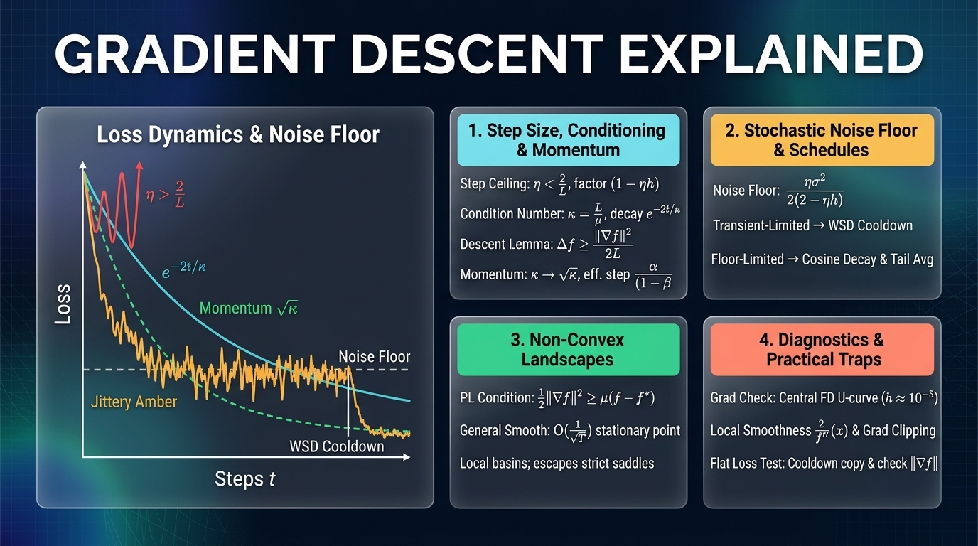
Prerequisites: derivatives of a function of several variables, the idea of an eigenvalue, and comfort reading a small table. Nothing from our Optimization Domain flagship is assumed; every place this piece touches it is given as a flagship section number so the theorist's version is one click away.
Reading path. The core is §1–§4 and it carries four ideas: a gradient step multiplies each curvature direction by , so the step has a ceiling and the slowest direction sets the clock; the condition number is the exponent's denominator, which is why doubling it doubles the steps; the descent lemma promises one specific decrease at one specific step and a line search is how you collect the rest; and momentum trades for by a theorem whose constants nobody uses. §5 is the stochastic regime where every training loop lives — the noise floor, and the schedule question that the floor decides. §6 is what survives of all this when the function is not convex, with the two smallest examples that separate the cases. §7 is three traps.
Companion Notebook
This article pairs with the companion script worked_numbers_companions.py — NumPy only, float64, CPU-only, one seed, about sixteen seconds — which ships with this piece beside the flagship's worked_numbers.py and prints every number quoted below; its A sections are this piece and its B sections are the companion on adaptive methods, Adam, Muon and Friends. A notebook, 00_gradient_descent.ipynb, is built from the A sections cell for cell once the prose is final, so that each quoted block is one runnable cell with its figure — the §A1 cell draws the four regimes of §1, contraction, exact landing, oscillation and divergence, as four panels. A section number in the form §A3 beside a block names the section that printed it; the numbers are verbatim.
One convention, once. is the function we minimise, its gradient, a minimiser, . is the smoothness constant: a bound on the magnitude of every curvature has — for a convex that is its largest curvature, and for a non-convex one it also bounds how negative the curvature gets. is the smallest curvature (the strong-convexity constant, when it is positive), and the condition number. is the step size, which the training world calls the learning rate; in §4, where momentum appears, the base step is written to keep it apart from , and the effective step on a constant gradient is . Gradient descent is the one line .
Three kinds of sentence. Every claim below is one of three things, and the text says which at the moment it is made: a theorem, true under the hypotheses stated; an identity under a model, exact for the toy it is computed on and only a guide elsewhere; or an observation at one seed, a number from one instance of one problem. The flagship grades the same claims L1–L3; here the words do the grading, and a reader who keeps the three apart will not turn a table into a theorem.
1. One coordinate: the step has a ceiling
Everything about gradient descent on a smooth problem is already visible on , one coordinate with curvature . The gradient is , so a step gives : each step multiplies the coordinate by the factor . That one factor is the whole theory of the step size.
§A1 One coordinate, f(x) = h x^2 / 2: each gradient step multiplies x by (1 - eta h); the step is stable iff eta h < 2
  eta*h    factor (1 - eta h)    x after 20 steps (x0 = 1)
   0.5        +0.500               9.5367e-07
   1.0        +0.000               0.0000e+00
   1.5        -0.500               9.5367e-07
   1.9        -0.900               1.2158e-01
   2.0        -1.000               1.0000e+00
   2.1        -1.100               6.7275e+00
  eta h = 1 is the Newton step (one step, exact); 1 < eta h < 2 oscillates and still converges; eta h = 2 bounces forever; eta h > 2 diverges
Read the table from the top. At the coordinate halves each step and is at after twenty. At the factor is zero: the step lands on the minimum exactly, because is Newton's step for a quadratic. At the factor is — the iterate overshoots the minimum and lands on the other side, half as far away, and the convergence is exactly as fast as at , only with alternating sign. At it still converges, slowly, bouncing. At the factor is and the iterate bounces between and forever. Past it grows.
So the step is stable on a direction of curvature if and only if , and the fastest convergence on that direction is at . This is the first thing the word "smoothness" means in practice. If is the largest curvature anywhere, the step is safe in every direction, and on a quadratic direction of curvature the step oscillates without converging (, the table's row) while any step above makes a nonzero component in that direction diverge — that is the theorem, and it is a theorem about a positive-curvature quadratic mode. On a general smooth function marks the end of the uniform descent guarantee, not where divergence must begin: §3's table has steps of and still decreasing a logistic loss, because the curvature along those steps was far below . This is why the theorems in §3 are stated at , and why a learning-rate sweep on a smooth problem has a cliff and not a slope on its right-hand side — the cliff is where the stiffest direction's is crossed. (The flagship's §1.4 is the formal definition; its §3.2 proves what the table shows.)
2. Two coordinates: the stiff one sets the step, the soft one sets the clock
Now give two coordinates, with curvatures and . The safe step is set by the stiff coordinate: . At that step the stiff coordinate is solved in one move (factor zero), and the soft coordinate — curvature — contracts by per step, which is barely less than one. The soft coordinate needs about steps to bring its loss below , because .
§A2 Two coordinates with curvatures 1 and kappa: the safe step 1/L is set by the stiff one, the iteration count by the soft one — linear in kappa
  kappa    iters to f < 1e-8 at eta = 1/L    ln(f0/eps)/(-2 ln(1 - 1/kappa))    iters at eta = 2/(L + mu)    ((kappa-1)/(kappa+1))^2t bound
     10              85                               95.5                           51                        50.1
    100             882                             1111.5                          559                       558.5
   1000            8860                            12312.0                         6160                      6159.1
  10000           88634                           134683.1                        67345                     67344.9
  the bound charges all of f0 to the soft coordinate; at eta = 1/L the stiff one, which holds kappa/(kappa+1) of f0, dies in one step, so the measured count sits under the bound by ln(1+kappa)/(-2 ln(1-1/kappa)) steps: 11, 230, 3453, 46050
Three things to take from the table, each of which survives into every later section.
The iteration count is linear in . Ten times the condition number, ten times the steps: , , . This is the sense in which is an exponent's denominator rather than a constant in front: the loss decays like , so the time to any fixed accuracy is proportional to . A problem whose curvatures span four orders of magnitude costs ten thousand times the steps of a well-conditioned one, at the same accuracy, with the same method. Nothing about the step size can fix this, because the step is pinned by the stiff direction and the clock is run by the soft one.
The bound is an upper bound, and the gap has a reason. The second column is the theorem's count, , and it is above the measurement by , , and steps. The theorem charges all of the initial loss to the slow direction, because for the worst function in the class that is where it is. Here the stiff coordinate holds of and is killed on the first step, so the slow direction starts with a -th of the loss the bound assumes, and saves e-foldings. When you compare a measured curve to a theorem and find the theorem pessimistic by a constant, the constant is usually the start; if it is pessimistic by a power of , you have the wrong function class (the flagship's §3.2 makes the same point on a fifty-dimensional example).
A better constant step exists, and it is not . The right-hand columns use , which balances the stiff and soft directions: both now contract by in magnitude, one from above and one from below, and the count drops by about a quarter — against at — and the bound is tight to the step, because the two directions now share the worst factor. This is the best any constant step can do on a quadratic; the factor is the one momentum (§4) improves on, and it does so by changing the method, not the step.
3. What the descent lemma promises, and how a line search collects more
The one inequality behind every rate in this piece is the descent lemma: if is -smooth — its gradient changes by at most per unit of distance — then one step of size decreases by at least . It is a statement about the worst possible curvature along the step, and on a real function the actual curvature along the step is usually smaller, so the actual decrease is usually larger. Here is the lemma on a logistic regression with two hundred points and five features, with a small ridge so that a minimiser exists — one seeded instance, so the ratios are observations and only the guarantee columns are the theorem:
§A3 The descent lemma on a logistic regression: one step of 1/L must cut the loss by at least ||g||^2 / (2L) — measured against the guarantee
  n = 200, d = 5, ridge 0.001: L <= lambda_max(X^T X)/(4n) + lambda = 0.2803, mu = 0.001, kappa <= 280
  f(w0) = 1.981075, ||grad f(w0)||^2 / (2L) = 0.587970 (the guaranteed decrease at eta = 1/L)
  eta * L    f(w0 - eta g)      actual decrease    lemma's guarantee at THIS eta: eta (1 - eta L/2) ||g||^2    decrease / own guarantee    decrease / the 1/L guarantee
   0.5       1.428574         +0.552500                            0.440977                         +1.253                      +0.940
   1.0       0.973392         +1.007682                            0.587970                         +1.714                      +1.714
   1.5       0.638469         +1.342606                            0.440977                         +3.045                      +2.283
   2.0       0.422451         +1.558624                   none (eta >= 2/L)                              -                      +2.651
   3.0       0.282509         +1.698566                   none (eta >= 2/L)                              -                      +2.889
   4.0       0.333676         +1.647399                   none (eta >= 2/L)                              -                      +2.802
  the lemma guarantees eta (1 - eta L/2) ||g||^2 at every eta < 2/L: largest at eta = 1/L, zero at 2/L, nothing beyond; each row beats its own guarantee, and 3/L and 4/L, which have none, still helped here because L bounds the worst curvature and this start is not in it
The lemma's promise depends on the step: at it is , largest at , zero at , nothing beyond. At the step decreased the loss by against a promise of : honoured with a factor of to spare. At the decrease of is times that step's own guarantee of — set it against the figure instead and it reads as a shortfall (), which is the wrong comparison, and the table shows both so the difference is visible. The steps of , and have no guarantee at all, decreased the loss more than any guaranteed step did, and is the first that did worse than . None of this contradicts §1. The constant is a bound on the curvature everywhere; the logistic loss has its largest curvature where the model is uncertain, at , and this starting point is confidently wrong on most examples, where the curvature is small. The step that is safe everywhere is not the step that is best here.
That is what a line search is for. Backtracking (Armijo's rule) tries a large step, checks whether the decrease is at least a fixed fraction of what a gradient step "should" buy, , and halves the step until it is. It costs extra loss evaluations and saves iterations:
§A4 Fixed step 1/L against backtracking line search (Armijo, start 10/L, halve) on the same logistic regression: iterations and loss evaluations to ||grad|| < 1e-6
  reference minimiser by damped Newton's method: f* = 0.2776084413, ||grad f(w*)|| = 1.1e-17, ||w*|| = 4.0477
  fixed eta = 1/L:             185 iterations,    185 gradients, f - f* = 3.31e-11
  backtracking (Armijo):        30 iterations,     30 gradients +     62 loss evaluations, f - f* = 1.31e-11, last accepted eta * L = 5.00
Thirty iterations against , at the price of sixty-two extra loss evaluations, and the last accepted step was — five times the step the theorem allows. On a problem where a loss evaluation is cheap relative to a gradient (a full forward pass against a forward-and-backward), that is a good trade; in a stochastic training loop it is not available in this form, because the loss you can evaluate is a noisy minibatch estimate, and a backtracking test passed on one minibatch says little about the function. Stochastic line searches do exist — Vaswani et al. (2019) run Armijo on the minibatch itself and prove rates under an interpolation assumption, Paquette & Scheinberg (2020) under a probabilistic model of the noise — and they are absent from the default recipe because their hypotheses are the price, not because the idea is impossible. This is the reason training uses a schedule (§5) where numerical optimization uses a line search: not because the line search is wrong, but because its test is unreliable on the noise a training loop can afford.
One remark on the reference. The minimiser in that block came from Newton's method, damped — a full Newton step from a far start, where the logistic Hessian is nearly the ridge alone, would fly off to a point with a loss of (we know, because the undamped version did, in the first run of this script). The flagship's §3.6 is why Newton is the method of choice when the Hessian is affordable, and this is the footnote: Newton's quadratic convergence is local, and the globalisation — a line search or a trust region — is not optional.
4. The two convex rates, and what momentum does to the square root
With the lemma in hand, the two theorems of the convex world follow in a few lines each (the flagship's §3.2 has both proofs). For a smooth convex , gradient descent at satisfies : the error falls like . If is also -strongly convex, : the error falls like , which is §2's clock again. Both bounds, on the logistic regression:
§A5 The two convex rates on the logistic regression: f(w_T) - f* against L||w0 - w*||^2 / (2T) and against (1 - mu/L)^T (L/2)||w0 - w*||^2
  ||w0 - w*||^2 = 37.4972
      T      f(w_T) - f*      smooth-convex bound L D^2/(2T)      strongly-convex bound (1 - mu/L)^T L D^2/2
       1       6.9578e-01           5.2545e+00                     5.2358e+00
      10       7.5227e-03           5.2545e-01                     5.0700e+00
     100       2.6374e-07           5.2545e-02                     3.6753e+00
    1000       5.5511e-17           5.2545e-03                     1.4728e-01
   10000       5.5511e-17           5.2545e-04                     1.5731e-15
  both bounds hold at every T and both are loose: the data term is itself strongly convex near w*, with a curvature the ridge-only mu = 0.001 does not see, so the measured gap falls far faster than either; 5.55e-17 is float64's floor
Both bounds hold at every , as they must, and both are loose by orders of magnitude. The reason is instructive and general. The theorem was told — the ridge — because that is the only strong convexity we can prove for a logistic loss, whose data term is merely convex (its curvature goes to zero for confidently classified points). Near this particular minimiser the data term's curvature is not zero at all; it is the dominant term, and the real local is in the tens, not the hundreds. The method sees the real function; the theorem sees the class. When a bound is this loose the fix is not a better theorem but a better class: tell the theorem what you know about the Hessian near the solution and the bound tightens. The bound, for its part, is the right rate for the worst convex function, which is flat near its minimum in a way this one is not.
Momentum. Two methods add a memory of the previous step. Heavy ball (Polyak 1964) is . Nesterov's method (1983) evaluates the gradient at the extrapolated point instead, . Both, with the right constants, replace by in the exponent:
§A6 Momentum on a 50-dimensional quadratic (curvatures log-spaced from 1 to kappa): GD, heavy ball, Nesterov — iterations to f < 1e-8
  kappa     GD iters    GD theory kappa ln(f0/eps)/2    heavy ball iters    Nesterov iters    sqrt(kappa) ln(.)
    100          866             1238                        75                 106                248
   1000         8907            13143                       263                 357                831
  10000        89579           143337                       990                1148               2867
  heavy ball at a constant unit gradient, alpha = 0.1, beta = 0.9: step / alpha after t = 1, 5, 10, 20, 60 steps = 1.000, 4.095, 6.513, 8.784, 9.982  (limit alpha/(1-beta) / alpha = 10.0)
Gradient descent grows by a factor of ten per decade of — , , — and the two momentum methods by a factor of about : heavy ball goes , , . At that is a ninety-fold saving. The constants that achieve it are tied to : heavy ball's are and , and is that value at , not a universal setting. Three honest qualifications, each from the flagship's §3.3: heavy ball's is a theorem about quadratics and can fail on other strongly convex functions, where Nesterov's holds for all of them; the heavy-ball rate's prefactor grows with (the flagship measures it), so the clean "" form one usually sees is not quite what is true; and in the stochastic regime of §5 momentum at a fixed effective step mainly averages the noise and does not change the noise floor.
What is a theorem without qualification is the last line. At a constant gradient, heavy ball's step grows to : at , ten times , and the table shows it getting there — after five steps, after ten, after sixty. When you set "momentum " in a training loop you have set the effective learning rate, in any direction the gradient agrees with itself, to ten times the number you typed. This is the single most useful fact in this section for a practitioner, and it is pure algebra.
5. The stochastic regime: a flat loss is a floor
A training loop does not see . It sees a minibatch gradient, , with a zero-mean noise whose variance shrinks with the batch size. On the one-coordinate problem of §1 that changes the recursion to , and the fixed point of the variance is no longer zero: shrinking by and adding each step, settles at , so the expected loss settles at a floor of — proportional to the step:
§A7 SGD on one noisy coordinate: the loss floor is proportional to the step — measured over 4000 chains against eta sigma^2 / (2 (2 - eta h))
    eta     measured E f (last 1500 steps)    theory eta sigma^2 / (2(2 - eta h))    ratio
   0.500           0.16677                           0.16667                    1.001
   0.100           0.02627                           0.02632                    0.998
   0.020           0.00504                           0.00505                    0.998
   0.004           0.00103                           0.00100                    1.023
  (eta = 0.004 has a time constant 1/(eta h) = 250 steps from a start of 3, so its last-half average still carries a little of the transient)
The formula is an identity for the model — one coordinate, additive noise of fixed variance — and the measurement agrees with it to at the three larger steps and to at the smallest, whose transient has not finished inside the averaging window; the parenthetical in the block is the whole of that gap. Halve the step, halve the floor; and halve the step, double the time constant of the transient. That is the whole trade-off of stochastic optimization in one line, and it is the same computation as the AR(1) process of our Probability Domain (§9.1 there) wearing a different costume — the flagship's §5.1 is the hand-off. Two consequences for reading a loss curve: a loss that is flat at a constant step is sitting on its floor, and is not converged in the sense of §1–§4 — drop the step and it will fall, by a factor the formula predicts, and go flat again lower; and a loss that is still falling at a constant step is in the transient of some slow direction. The two look the same on a log plot. The one test that separates them is to cool the step down on a copy of the checkpoint and see whether the loss drops.
Schedules. Because the step wants to be large for the transient and small for the floor, every training recipe changes it over the run. Which schedule is best is not a universal question, and the smallest model that shows why is a quadratic with many directions, curvature , noise proportional to curvature, on which the expected loss under any step sequence can be computed exactly, coordinate by coordinate, with no sampling — the noisy quadratic model of Zhang et al. (2019), which the flagship's §5.4 uses at a larger size. Here are four schedules in two regimes, same steps, same step ceiling, differing only in how many slow directions the problem has:
§A8 Schedules on a noisy quadratic, curvatures 1/i, exact expectations: constant, cosine, warmup-stable-decay, 1/sqrt t — in a transient-limited and a floor-limited run; tail averaging, simulated
  transient-limited: d = 1000, slowest time constant 1/(eta h_min) = 1000 = T; h_i = 1/i, noise c/B = 0.015625, T = 1000; expected loss at t = 200, 800, 1000:
    constant eta_max                   0.38268     0.07744     0.05890
    cosine to 0                        0.39027     0.11940     0.11547
    WSD (80% const, 20% linear)        0.38268     0.07744     0.04382
    1/sqrt(t)                          1.20131     0.86872     0.81780
    constant eta_max/10                1.34216     0.70706     0.61389
  floor-limited: d = 200, slowest time constant 200 = T/5; h_i = 1/i, noise c/B = 0.015625, T = 1000; expected loss at t = 200, 800, 1000:
    constant eta_max                   0.05254     0.02839     0.02837
    cosine to 0                        0.05164     0.00492     0.00345
    WSD (80% const, 20% linear)        0.05254     0.02839     0.00639
    1/sqrt(t)                          0.49647     0.25256     0.22058
    constant eta_max/10                0.61359     0.15794     0.11230
  d = 1000, constant eta_max, 20 simulated runs: last-iterate loss 0.05628 +- 0.00158; loss of the average over the last 25% 0.04414 +- 0.00023
Read the two halves against each other.
In the transient-limited run — a thousand directions, the slowest with a time constant equal to the whole budget — the constant step is still working on the slow directions at the end, and anything that gives up the large step early loses: cosine finishes at , twice the constant step's , because it spent the middle of the run at a step too small for the transient. Warmup-stable-decay (constant for , then linear to zero) is identical to the constant schedule until step — the same curve — and then the cooldown collapses the floors to finish at , the best of the four. This is the mechanism Hägele et al. (2024) found at 124M–1B parameters and the reason the cooldown has displaced cosine in many recipes.
In the floor-limited run — two hundred directions, the slowest done in a fifth of the budget — the ranking reverses. The constant step reaches its floor by step and sits there; now the run is all floor, and the schedule that spends the most time at small steps wins: cosine finishes at , WSD at , nearly twice as high, because its cooldown is only a fifth of the run. Same problem family, same step, same budget; the opposite answer. The variable that decides is the ratio of the slowest time constant to the horizon, and no schedule is best without knowing it. is last in both regimes on the last iterate — it is the schedule the convex theory prescribes for the averaged iterate, and the theorem is about , not .
Averaging is the other way to pay the floor down: the last line simulates the constant-step run and averages the iterates over its last quarter. The average's loss, , equals what the cooldown reached, with no change to the step at all. That is Polyak–Juditsky averaging, the mechanism of stochastic weight averaging, and of schedule-free methods that maintain the average on-line. On the quadratic it is a theorem (the average of an AR(1) has smaller variance by its window); as a statement about a deep network's loss it is a measurement, and the flagship's §5.4 grades it.
6. Non-convex: what survives, on the two smallest examples
The two rates of §4, and every sentence above with the word global in it, assumed convexity — local minima are global, the first-order condition is sufficient, the chord lies above the function. Not everything did: the descent lemma of §3 and the noise-floor identity of §5 never used it, and the inventory at the end of this section says which is which. A neural network's loss is convex in none of these senses. What survives is more than one might expect and less than the convex reader hopes, and two one-dimensional functions show the boundary:
§A9 Non-convex, two ways: f(x) = x^2 + 3 sin^2 x (PL: every stationary point is the minimum) against f(x) = x^4/4 - x^2/2 (two minima, one saddle)
  PL example, eta = 1/L = 1/8, 200 steps:        start     final x      final f      |f'(x)|
                                                 -3.0     +0.00000     0.00e+00     0.0e+00
                                                  2.0     +0.00000     0.00e+00     0.0e+00
                                                  5.0     +0.00000     0.00e+00     0.0e+00
                                                 10.0     +0.00000     0.00e+00     0.0e+00
  double well, eta = 0.1, 200 steps:                start     final x      final f
                                                 -2.0     -1.00000     -0.25000
                                                 -0.5     -1.00000     -0.25000
                                                  0.0     +0.00000     +0.00000
                                                  0.5     +1.00000     -0.25000
                                                  2.0     +1.00000     -0.25000
                                                  3.0     +1.00000     -0.25000    (first steps +0.6, +0.6384, +0.6762)
                                                  4.0     -1.00000     -0.25000    (first steps -2, -1.4, -1.266)
                                                  5.0     overflow     overflow    (first steps -7, +26.6, -1853)
  f(0) = 0 is a stationary point of the double well and a start of exactly 0 stays there forever; the tested starts with |x0| <= 2 fall to the NEARER minimum f = -0.25; x0 = 4 overshoots into the FAR well and x0 = 5 diverges — f''(x) = 3 x^2 - 1 passes 2/eta = 20 at |x| = 2.65, so eta = 0.1 is a step that is safe only near the wells (the local-smoothness trap of A11)
The first function, , is not convex — its second derivative is negative on intervals — and yet gradient descent at lands on the global minimum at zero from the four tested starts — and, by the theorem below, from every start. It satisfies the Polyak–Łojasiewicz inequality, with (Karimi, Nutini & Schmidt 2016): the gradient is never small away from the minimum, so every stationary point is the minimum, and the linear rate of §4 holds with no convexity at all (the flagship's §6.4). Over-parameterised networks near their initialisation are the setting in which a condition of this kind has been shown to hold, and it is the honest reason "gradient descent finds a global minimum of a wide network" can be a theorem.
The second function, , has two minima at and a saddle — a local maximum, in one dimension — at zero. From the tested starts with , gradient descent goes to the nearer minimum, and a start of exactly zero stays at zero forever, because the gradient there is zero. That sentence is about these starts at this step, not a theorem: from the first step overshoots to and the run ends in the far well, and from it goes and diverges, because the curvature passes the step's ceiling at — §7.2's trap, met early. Both minima have the same loss here, so a run that converges succeeds; make the right well deeper and a start at still goes left. This is the general situation, and the general theorem is correspondingly weaker. For an -smooth that is bounded below, gradient descent at satisfies — summing the descent lemma over steps is the whole proof. Read it for what it says: it is a statement about the best iterate so far. Some iterate is nearly stationary, at the rate on the gradient norm, and the stochastic version (Ghadimi & Lan 2013; the flagship's §6.2) returns a randomly chosen iterate for the same reason. It does not say that the sequence converges to a single stationary point — that needs assumptions beyond smoothness. From a random start gradient descent also avoids the strict saddles with probability one — a theorem with three hypotheses, each needed: every saddle is strict (it has a direction of negative curvature), the step is small enough (), and the start is drawn from a distribution with a density, so that the measure-zero set of starts that converge to a saddle is never hit (§6.3 there states it); it does not find the global minimum, and no first-order method can promise to (§6.1).
So the practitioner's inventory: the step ceiling of §1 survives, locally; the clock of §2 survives, with now the local condition number at the minimum you reach; the descent lemma of §3 survives verbatim, because it never used convexity; the stochastic floor of §5 survives exactly on the quadratic model and only approximately near a stable non-convex minimum, where the local quadratic is the model; and the rates of §4 survive only under a PL-type condition, which is a property you can sometimes verify and more often cannot. What dies is the word global.
7. Where intuition breaks, and what to do instead (deeper reading)
7.1 — "My gradient is right because the loss went down." The loss can go down under a wrong gradient, and it can even pass a sufficient-decrease test: on at , an implementation that returns instead of the true gradient still cuts the loss by at a unit step, more than the Armijo threshold of it would be checked against. Any vector with a positive inner product with the true gradient is a descent direction, so a convincing decrease is evidence of descent, not of correctness. The test is a central finite difference, and its result is read as a U:
§A10 Checking a gradient by central finite differences: the relative error is U-shaped in the step h (truncation on the right, rounding on the left)
  first, why 'the loss went down' is not the test: f(x) = x^2/2 at x = 1 has gradient 1; a WRONG gradient of 0.8 at step 1 lands at x = 0.2 and cuts the loss by 0.480, more than the Armijo threshold (1/2) eta g_hat^2 = 0.320 computed with the wrong gradient — the sufficient-decrease test accepts a wrong gradient; the finite-difference check below is the test
        h       max relative error over 5 coordinates
     1e-01         2.14e-03
     1e-02         2.14e-05
     1e-03         2.14e-07
     1e-04         2.14e-09
     1e-05         5.51e-11
     1e-06         3.15e-10
     1e-07         6.02e-09
     1e-08         1.10e-07
     1e-10         5.49e-06
From down to the error falls by a factor of a hundred per decade — the central difference's truncation error is — reaches at , and then rises, because the difference of two nearly equal losses loses digits to float64's rounding at a rate of . The minimum, near for a loss of order one, is the resolution of the test; a gradient that agrees to there is right, and a disagreement of at is the test failing, not the gradient. Use the elbow, not the smallest you can type.
7.2 — "The learning rate was fine at the start." Smoothness is a global constant in the theorems and a local quantity in a run. On the curvature is at , at and at , so the local step ceiling is , and — and the same step is under it from one start and over it from another:
§A11 Smoothness is local: gradient descent on f(x) = x^4 from x0 = 1 — eta = 0.1 converges, eta = 0.6 diverges, and clipping the gradient to norm 1 rescues it
  eta = 0.1, x0 = 1         : x at t = 0..5 = +1, +0.6, +0.5136, +0.4594, +0.4206, +0.3909;  x at t = 10 = +0.3034
  eta = 0.1, x0 = 2         : x at t = 0..5 = +2, -1.2, -0.5088, -0.4561, -0.4182, -0.3889;  x at t = 10 = -0.3025
  eta = 0.1, x0 = 3         : x at t = 0..5 = +3, -7.8, +182, -2.412e+06, +5.613e+18, -7.075e+55;  x at t = 10 = overflow
  eta = 0.05, x0 = 2        : x at t = 0..5 = +2, +0.4, +0.3872, +0.3756, +0.365, +0.3553;  x at t = 10 = +0.3163
  eta = 0.6, x0 = 1         : x at t = 0..5 = +1, -1.4, +5.186, -329.5, +8.584e+07, -1.518e+24;  x at t = 10 = overflow
  eta = 0.6, x0 = 1, clip 1.0: x at t = 0..5 = +1, +0.4, +0.2464, +0.2105, +0.1881, +0.1721;  x at t = 10 = +0.1292
  f''(x) = 12 x^2, so the local step ceiling 2/f''(x) is 0.167 at x = 1, 0.042 at x = 2, 0.019 at x = 3: eta = 0.1 is under the ceiling at x0 = 1 and converges, over it at x0 = 2 and still recovers (the overshoot lands at -1.2, inside the safe region), over it at x0 = 3 and diverges; eta = 0.6 is already 3.6x over the ceiling at x0 = 1, and every overshoot lands where the curvature is larger still; no single eta is safe from every start, and clipping bounds the step's length instead
  2/f''(x) is the contraction threshold of the LOCALLY LINEARISED map, not an overshoot threshold: the exact x^4 update is x (1 - 4 eta x^2), whose sign flips only at eta = 1/(4 x^2) = 0.0625 at x = 2, above the local ceiling 1/24 = 0.0417; eta = 0.05 from x0 = 2 is over the ceiling and lands at +0.4 with no overshoot, eta = 0.1 crosses to -1.2 and still shrinks |x|, so the run recovers
At the run from converges, the run from overshoots to and recovers, and the run from goes and overflows a double before step ten: the learning rate that was fine from one start is not fine from another. One precision about the ceiling. is the contraction threshold of the locally linearised map; on a non-linear function it is neither an exact overshoot threshold nor a universal divergence threshold. For the update is , which changes sign only at — at , above the local ceiling — so from is over the ceiling and lands at with no overshoot (the block's fourth row), while crosses to but still shrinks , which is why that run recovers. At the step is already times over the ceiling at — it was never locally safe, which is the honest reading of that row — and each overshoot lands where the curvature is larger still. A function with no global has no step that is safe from every start. Two remedies, both standard: a decreasing step, which the theorems of §5 wanted anyway; and gradient clipping, which caps the gradient's norm — here at — so that the step's length is bounded whatever the curvature does. The clipped run at the same converges. Clipping is not a trick for exploding gradients; it is the practitioner's substitute for a smoothness constant the problem does not have.
7.3 — "A flat loss means it converged." §5. At a constant step under noise, flat means floor. The test is a cooldown on a copy of the checkpoint; if the loss drops, you were on a floor, and the drop's size tells you the noise level through the §A7 formula. A flat deterministic loss — full batch, no noise — is not a certificate of optimality either: it indicates a stationary point, and §6's double well sits at exactly zero forever from a start of , with one unit away. Check the gradient norm, and where convexity or a PL condition holds, use it to turn "stationary" into "optimal"; without one of them, flat means stationary and no more.
What to take away
- A gradient step multiplies each curvature direction by . Stable iff — a theorem for a quadratic direction; exact at ; oscillating but convergent in between; bouncing forever at exactly . On a general smooth function is where the guarantee ends, not where divergence must start; the step is capped by the stiffest direction's , which is why a learning-rate sweep has a cliff on its right.
- The condition number is an exponent's denominator. At the slow direction contracts by per step, so the step count is linear in : , , . The bound sits above the measurement by a constant that is the start, not slack.
- The descent lemma promises at and no more; a line search collects what the local curvature allows. Thirty iterations against on a logistic regression, at the price of sixty-two loss evaluations. Training uses schedules instead because a backtracking test on one minibatch is unreliable; stochastic line searches exist and carry extra hypotheses.
- Momentum turns into , at constants tied to that nobody sets. Heavy ball at : steps against . What is true at any is that the effective step on a steady gradient is — ten times at .
- Under noise the loss has a floor proportional to the step, , measured to within where the transient has finished and at the smallest step, where it has not. Flat is not converged; the test is a cooldown on a copy.
- No schedule is best without knowing whether the run is transient-limited or floor-limited. The constant-then-cooldown schedule wins by a factor of over cosine when the slowest direction's time constant equals the budget, and loses by a factor of when it is a fifth of it. Averaging the last quarter of a constant-step run buys what the cooldown buys.
- Non-convexity kills the word global and little else. The step ceiling, the clock and the descent lemma are local statements and survive, and the noise floor survives on the local quadratic; the general guarantee is that the best iterate is nearly stationary, not that the sequence converges; the linear rate survives under PL; shows the general case — the nearer minimum from the tested nearby starts, the far well from , divergence from , and a saddle that holds a start of exactly zero forever.
Where to go next
The companion script worked_numbers_companions.py prints every number above in its A sections, and its B sections carry the second companion of this package, Adam, Muon and Friends, which takes the one-coordinate picture of §1 and asks what happens when the step is normalised per coordinate (Adam), orthogonalised per matrix (Muon), or decoupled from the weight decay (AdamW) — and which of the resulting claims are theorems.
This package's flagship, The Optimization Domain, takes each section here one level down and then forward to the theorem behind a training claim: §1 for convexity and the one pathology it leaves, §3.2–§3.4 for the two rates, acceleration and Nesterov's lower bound, §5 for the stochastic regime at full size — batch size, variance reduction, the five schedules, warmup, weight decay as an equilibrium — and §6–§7 for what a non-convex guarantee is allowed to say and which claims about networks have one. Our Probability Domain is where the noise in §5 comes from, and its companion Probability Theory Explained is the shortest route to the AR(1) computation behind the floor.
For deeper reading: Boyd & Vandenberghe's Convex Optimization (2004) is the standard first book and is free online; Nesterov's Lectures on Convex Optimization (2nd ed., 2018) has the rates and lower bounds of §4 as theorems with proofs; Bubeck's Convex Optimization: Algorithms and Complexity (2015) is the shortest honest route to the same; Nocedal & Wright's Numerical Optimization (2nd ed., 2006) is where line searches, trust regions and the globalisation of Newton's method live; and Bottou, Curtis & Nocedal's Optimization Methods for Large-Scale Machine Learning (SIAM Review, 2018) is the survey that connects §5 to the training loop.
We build agent systems and practitioner tooling at Artifocial — see our apps, including Alarmly.