Probability Theory Explained: Sample Spaces, Random Variables, and the Expectation You Already Optimise

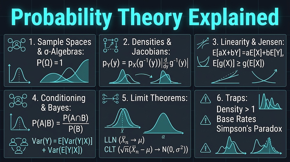
Prerequisites: comfort with sums, integrals and the idea of a function; nothing about measure theory (§3.1, which is marked optional, is the one place that uses it beyond the vocabulary of §1). If you want the machinery before the intuition, start at §2 and come back to §1.

Reading path. On a first pass the core is §1–§5, and it carries five ideas: a probability is a function on questions, a random variable is a function and its distribution is what that function does to the probability, expectation is a weighted average that is linear whatever the dependence, conditioning is a projection and the conditional mean is therefore the best predictor by theorem, and the two limit theorems are what entitle you to average anything at all. §6 (the traps) is where the ideas earn their keep and can be read on its own on the day one of them bites. The flagship this piece accompanies, The Probability Domain, takes every definition here to its measure-theoretic statement and then to the theorem under a training claim; this piece stops at the point where the definition becomes usable and tells you where in the flagship the rest is.

Companion Notebook

This article pairs with 00_probability_from_scratch.ipynb — pure NumPy and Matplotlib, CPU-only, every figure inline — which ships with this piece and carries the same material in runnable form: the three Bertrand measures sampled side by side, the density that exceeds one, the change of variables with and without its Jacobian, the dice experiment that separates linearity of expectation from additivity of variance, the orthogonality of the regression residual, the cross-entropy bowl with its minimum at the true conditional probability, the running means that converge and the two that never will, and the great circle conditioned two ways. Every table and printed block quoted below is copied (with repeated or trailing annotations trimmed) from the output of worked_numbers_companions.py (sections §A1–§A18), the script the notebook is built from, — Python 3.14.5, NumPy 2.5.3, float64, seed 20261029 fixed at the top — so a re-execution reproduces every one of them; a few values in the prose are derived from those outputs or from the closed forms on the page and are marked where they appear.

One convention, once. We write $P(A)$ for the probability of an event, $p(x)$ for a density or a mass function, and $\mathbb E[X]$ for an expectation. The distinction between $P$ and $p$ is the subject of §2 and is the single most common source of error in probabilistic code, so it is kept visible throughout.

1. A probability is a function on questions

Most introductions begin with "the probability of an event is the fraction of times it happens in the long run", and then spend three chapters apologising for that sentence. Let us begin somewhere that needs no apology, because it is both correct and simpler.

Roll two dice. Write down everything that could happen: $(1,1), (1,2), \dots, (6,6)$ — thirty-six outcomes. That list is the sample space $\Omega$. A probability is a function that assigns a number in $[0,1]$ to subsets of $\Omega$ — to events, which are the questions you might ask, like "the sum is 7" or "the first die shows 6" — subject to three rules: nothing has negative probability, the whole space has probability $1$, and the probability of a union of countably many events that cannot happen together — finitely many, or infinitely many that can be listed as $A_1, A_2, A_3, \dots$ — is the sum of their probabilities. On the dice, every outcome gets $\tfrac1{36}$, and the rules do the rest:

§A1 |Omega| = 36;  P(sum = 7) = 6/36 = 0.1667;  P(sum = 2) = 1/36 = 0.0278

Three things in that paragraph are doing more work than they appear to.

First, probability is assigned to events, not to outcomes. On the dice these coincide — each outcome is an event of one point — but the moment the sample space is continuous they come apart: the probability of a dart landing at exactly one point of a board is $0$, and yet the dart lands somewhere. Every probability you will ever compute is the probability of a set, and §2 is about what happens when you forget that.

Second, the list of questions is itself a choice. Suppose you are told only the sum of the two dice. Then "the sum is 7" is a question you can answer, and "the first die is 6" is not — the outcomes $(1,6)$ and $(6,1)$ both have sum $7$ and you cannot tell them apart. The collection of questions you can answer from the sum is smaller than the full collection of $2^{36}$ subsets:

§A1 blocks of sigma(sum): 11 (one per value 2..12); events you can ask about given only the sum: 2^11 = 2,048 of the 2^36 = 68,719,476,736 subsets
    'first die is 6' is NOT in sigma(sum): it splits the block sum=7 = [(1, 6), (2, 5), (3, 4), (4, 3), (5, 2), (6, 1)]

A collection of events that contains $\Omega$ and is closed under complement and under countable unions is called a σ-algebra, and the one generated by a piece of information — "the sum" — is exactly the list of questions that information lets you answer. That is the whole intuition for a word that frightens people: a σ-algebra is a list of questions you are allowed to ask, and conditioning on information means restricting yourself to that list. Nothing more is needed to read the rest of this piece; the flagship's §1.3 takes the same idea to filtrations and martingales, and shows that "the model has seen the first $t$ tokens" is a σ-algebra statement too.

Third, "countable" in the third rule is not pedantry. Toss a fair coin until the first head. The event "a head eventually appears" is the union of the disjoint events "the first head is on toss $k$" for $k = 1, 2, 3, \dots$ — infinitely many of them — and its probability is the sum of theirs:

§A2 sum_{k>=1} 2^-k over k=1..60 = 1.0000000000000000  -> 1 (countable union of disjoint events 'first head at toss k')
    P(all tails in first n): n=10: 0.000977   n=30: 9.313e-10   n=100: 7.889e-31   -> 0 ; the event 'all tails forever' has probability 0 but is NOT empty

Finite additivity already gets you most of the way: $P(\text{a head within the first } n \text{ tosses}) = 1 - 2^{-n}$ is a finite sum, and because "a head eventually" contains each of those events, its probability is at least $1 - 2^{-n}$ for every $n$ — so once that event is on the list of questions, the rules applied to finite unions alone force its probability to be $1$.

What the countable rule buys is more basic. It is what gives a probability on infinite coin sequences its one canonical form: a function assigning $2^{-n}$ to every pattern of $n$ tosses extends to a probability on the set of all infinite sequences in exactly one way — so that an event like "infinitely many heads", which no finite prefix decides, gets one determined number (here $1$) instead of any value in $[0, 1]$ — only because the rule holds for countable unions. And it gives continuity: if events $A_1 \subseteq A_2 \subseteq \dots$ grow towards their union $A$, then $P(A) = \lim_n P(A_n)$, which is the licence behind every "in the limit" statement in the rest of this piece. Without the countable rule, strange objects are allowed — there are finitely additive "uniform" probabilities on the whole numbers $\{1, 2, 3, \dots\}$ that give every single number probability $0$ and the whole set probability $1$, so the parts sum to $0$ while the whole is $1$.

The complementary event — all tails, forever — is a perfectly good outcome that has probability $0$. It is not impossible; it is null. The distinction between "impossible" and "probability zero" sounds like philosophy until you meet a continuous random variable, where every individual outcome has probability zero and one of them happens anyway. "Almost surely" means "except on a null set", and every convergence claim about a training run that says "the loss converges" is, when it is a theorem at all, usually a claim of that kind (the alternatives — convergence in probability or in mean square — are the modes §5 ends on).

1.1 "Random" is not a property of a set

Here is the puzzle that shows why the definition has to be this careful. Draw a chord of a circle "at random". The equilateral triangle inscribed in the circle has side $\sqrt 3$ (for a unit circle); how often is the chord longer than that? There are three natural ways to draw a random chord, and they do not agree:

§A3 (a) two uniform endpoints        P(L > sqrt3) = 0.3333   (theory 1/3)
    (b) uniform distance to centre   P(L > sqrt3) = 0.4997   (theory 1/2)
    (c) uniform midpoint in the disc P(L > sqrt3) = 0.2502   (theory 1/4)

This is Bertrand's paradox (1889), and it is not a paradox. "Uniform" is not a property of the set of chords. It is a property of a probability function on that set, and the set of chords has three equally natural ones. Pick uniform endpoints and the answer is $\tfrac13$; pick a uniform distance from the centre and it is $\tfrac12$; pick a uniform midpoint and it is $\tfrac14$. Each is correct for its probability function — its measure, in the standard word, which we use from here on. The question "what is the probability a random chord is long?" has no answer until "random" has been given a measure, and then it has exactly one.

Carry that into your own work. "Sample uniformly from the data manifold", "a random initialisation", "an uninformative prior" — each of those phrases either specifies a probability function or it has not yet said anything, and two engineers who fill in the blank differently will disagree about a number without either of them having made an arithmetic mistake. The flagship's §0 and §10.1 return to this for priors; the lesson here is only the discipline: when you say "random", say which measure.

2. A random variable is a function, and a density is not a probability

A random variable is a function from the sample space to numbers. On the dice, "the sum" is the function $X(i, j) = i + j$. On these dice, with every subset measurable, that is the entire definition; in general there is one more requirement — that every question "$X \in B$" (for every interval $B$, say) be on the σ-algebra's list of allowed questions, which is called measurability, and is what lets $P(X \in B)$ be defined at all. It is automatic when the σ-algebra is the list of all subsets, as it is on the dice; it is not automatic on a finite space as such — with only $\sigma(\text{sum})$ available, "the first die is 6" is not a measurable question (§1), so the first die is not a random variable for that information. The definition resolves a confusion that costs people years: a random variable is not "a variable that is random". It is an ordinary, deterministic function; the randomness lives in which point of $\Omega$ you were handed, and the function just reports a number about that point.

Its distribution is what the function does to the probability: $P(X \in B)$ is the probability of the set of outcomes that $X$ sends into $B$. The dice sum is $7$ on six of the thirty-six outcomes, so $P(X = 7) = \tfrac{6}{36}$. The probability was always on $\Omega$; the distribution of $X$ is that probability pushed forward through the function. This is why you can have two different random variables with the same distribution (the first die and the second die), and why "$X$ and $Y$ have the same distribution" is a much weaker statement than "$X = Y$" — a distinction with a practical cousin: two samplers whose one-dimensional histograms match coordinate by coordinate can still have different joint distributions (the distribution of all coordinates together), which is the trap generative-model evaluation falls into whenever it compares marginal histograms and concludes the samplers are the same.

2.1 Discrete, continuous, and the one object that covers both

For a discrete random variable the distribution is a probability mass function $p(x) = P(X = x)$, and it is a genuine probability. For a continuous one, $P(X = x) = 0$ for every $x$, so there is nothing to tabulate. What survives is the cumulative distribution function $F(x) = P(X \le x)$, which is defined for every random variable whatsoever, and — when it is smooth — its derivative, the probability density function $p(x) = F'(x)$. The density answers a different question from the mass function: not "how likely is $x$" but "how much probability per unit length sits near $x$". The probability of an interval is the integral of the density over it; the probability of a point is zero.

This is why a density can exceed one, and why that is not an error:

§A4 sigma = 1.0  : density at 0 =    0.399;  P(|X| < 0.01) = 0.0080
    sigma = 0.1  : density at 0 =    3.989;  P(|X| < 0.01) = 0.0797
    sigma = 0.01 : density at 0 =   39.894;  P(|X| < 0.01) = 0.6827
    the density exceeds 1 as soon as sigma < 1/sqrt(2 pi) = 0.3989; a probability never does

A Gaussian with standard deviation $0.01$ has density $39.9$ at its centre and probability $0.68$ of landing within $0.01$ of it. The density is a rate; multiply it by a width to get a probability. The practical consequences are immediate and they are the ones people get wrong:

• A likelihood is a density, so a log-likelihood can be positive. A model reporting $\log p(x) = +3.2$ on a continuous input is not broken. Bits-per-dimension figures for image models exist because pixels are discrete — 8-bit integers — so the continuous density is converted into a code length for those discrete values (by dequantisation: add uniform noise to the integer pixels, and the continuous log-density, averaged over that noise, is a lower bound (Jensen again, §3.2) on the discrete log-probability; Theis, van den Oord & Bethge 2016). That is why a bits-per-dimension figure is a genuine probability-based quantity, comparable across models, while a raw log-density on integer pixels is not — a continuous model can pile density onto the integers and report as large a log-density as it likes.
• A density is not invariant to how you measure $x$. Change units from metres to millimetres and the density is divided by $1000$ — it is now probability per millimetre instead of per metre; the probability of any event is unchanged. §2.2 makes this exact.
• Comparing a density to a probability is a type error. A classifier's softmax output is a probability mass function and lives in $[0,1]$. A normalising flow's output is a density and does not. Code that clips a "probability" to $[0,1]$ before taking its log is correct for one and silently wrong for the other.

2.2 Change of variables: where the Jacobian comes from

If $Y = g(X)$ for a smooth, invertible $g$, the density of $Y$ is not $p_X(g^{-1}(y))$. It is

and the second factor is not decoration. The density is probability per unit length, and $g$ stretches or compresses lengths; the derivative is the local stretch factor. Here is what happens when you forget it, with $X \sim \mathcal N(0,1)$ and $Y = e^X$:

§A5 max |hist - phi(log y)/y| over 120 bins = 0.0095   (sampling noise);  max |hist - phi(log y)| (Jacobian forgotten) = 0.4521
    integral of phi(log y)/y dy over (0, 60] = 1.0000;  integral of phi(log y) dy = 1.6471

The correct density matches the histogram to within sampling noise — the histogram is normalised by the whole sample of two million and the bin width, not by the $96\%$ of it that falls inside the plotted range, which is the normalisation density=True would silently apply — and integrates to one. The "density" with the Jacobian dropped is off by $0.45$ at its worst point and integrates to $1.65$ — it is not a probability distribution at all. In higher dimensions the derivative becomes the absolute determinant of the Jacobian matrix, and that term — $\log|\det J|$ — is the one every normalising flow computes and every flow architecture is designed to make cheap. It is not a modelling choice. It is the change-of-variables formula, and a flow is a learned $g$ whose Jacobian you can afford.

The same line explains why reparameterisation works in a VAE: writing $z = \mu + \sigma\epsilon$ with $\epsilon \sim \mathcal N(0, I)$ is a change of variables from $\epsilon$ to $z$, so an expectation over $z$ becomes an expectation over $\epsilon$ and the parameters move inside the integrand, where a gradient can reach them. The flagship's §2.3 and §3.3 state the theorem that licenses that move and the kind of loss where it fails.

3. Expectation is a weighted average, and it is linear whatever the dependence

The expectation of a random variable is its probability-weighted average: $\mathbb E[X] = \sum_x x\,p(x)$ for a discrete $X$, $\int x\,p(x)\,dx$ for a continuous one. For a function of $X$ there is no need to find the distribution of $g(X)$ first — $\mathbb E[g(X)] = \sum_x g(x)\,p(x)$, a fact textbooks call the law of the unconscious statistician because everyone uses it without noticing. The expectation of the dice sum is $7$; the expectation of a fair coin's indicator is $\tfrac12$; the expectation of your loss over the data distribution is the thing your training loop is trying to minimise, and the training loss on a batch is a sample average standing in for it.

Expectation has one property that is more useful than all the others combined, and it is the one most often hedged with a condition it does not need — independence:

Linearity. $\mathbb E[aX + bY] = a\,\mathbb E[X] + b\,\mathbb E[Y]$, for any random variables $X$ and $Y$ on the same space whose expectations are finite — independent, dependent, identical, it does not matter. (Finiteness is the one hypothesis: §3.3 meets a variable with no expectation, and for it the right-hand side is not even defined.)

Variance does not have this property; $\mathrm{Var}(X + Y) = \mathrm{Var}(X) + \mathrm{Var}(Y)$ needs $X$ and $Y$ uncorrelated. Here is the difference on the dice, once with two independent dice and once with the same die counted twice:

§A6 independent dice: E[D1+D2] = 6.9973 (= 3.5+3.5);  Var(D1+D2) = 5.8344 (= 2 * 35/12 = 5.8333)
    same die twice:   E[D1+D1] = 6.9998 (= 3.5+3.5);  Var(D1+D1) = 11.6925 (= 4 * 35/12 = 11.6667) — linearity held, additivity of variance did not

The expectation of the sum is $7$ in both cases. The variance doubles in one and quadruples in the other. This is the reason "the expected number of ..." problems that look impossible are usually one line: write the count as a sum of indicators, take the expectation of each, add — the indicators can be as dependent as they like. It is also the reason a mini-batch gradient is an unbiased estimate of the full gradient (linearity of expectation over which examples were sampled) while its variance depends on how the examples co-vary and on the batch size. Unbiasedness is free; variance you pay for.

3.1 Why the integral has to be Lebesgue's, in one picture (optional)

This subsection can be skipped on a first pass; the one sentence a practitioner needs is the bold one at its end. You may have heard that "real" probability uses the Lebesgue integral and wondered whether that matters to you. Here is the entire idea, and then the one place it matters.

Riemann's integral slices the domain: cut the $x$-axis into small intervals, multiply each interval's width by the function's height there, add. Lebesgue's integral slices the range: for each value $y$ the function might take, measure the set of $x$ where the function is about $y$, multiply by $y$, add. For a continuous function on an interval the two agree. For the indicator of the rationals in $[0,1]$ — a function that is $1$ on a dense set and $0$ on another dense set — Riemann's upper sums are all $1$ and his lower sums all $0$, so the integral does not exist; Lebesgue asks "how big is the set of rationals?", gets the answer $0$ (a countable set of points), and returns $0$.

Slicing by value is the move that lets you integrate over any probability space whatsoever, because "measure the set where $X$ is about $y$" is exactly what a probability does, and it is why $\mathbb E[X]$ can be written as one symbol for a dice sum, a Gaussian and a random function alike.

The place it matters to a practitioner is the limit theorems. Monotone convergence and dominated convergence are the two statements about when $\lim \mathbb E[X_n] = \mathbb E[\lim X_n]$ — when a limit and an expectation can be swapped — and Fatou's lemma is the one-sided bound that survives when neither applies ($\mathbb E[\liminf X_n] \le \liminf \mathbb E[X_n]$ for non-negative $X_n$: the expectation of the limit can be smaller than the limit of the expectations, never larger); together they are the hypotheses under every "gradient of an expectation" in a training loop, including the one that makes REINFORCE unbiased and the one that makes the reparameterisation trick valid.

The flagship's §3 gives them with the counter-example that separates them; here it is enough to know that swapping a limit and an expectation is a theorem with a condition, not an algebraic identity, and that the condition fails for the pathwise gradient — differentiating the loss along the sample, as reparameterisation does — of the 0–1 loss and every other piecewise-constant metric — accuracy, top-$k$, exact match — whose gradient is zero almost everywhere while the expectation's gradient is not. A score-function estimator (REINFORCE) differentiates the density rather than the loss and stays unbiased under conditions of its own, so the two estimators fail in different places; the flagship's §3.3 runs both on the same loss.

3.2 Jensen's inequality, and why every variational bound is a bound

If $g$ is convex, $\mathbb E[g(X)] \ge g(\mathbb E[X])$. If $g$ is concave, the inequality flips. That is Jensen, and the log is concave:

§A5 E[Y] = e^(1/2) = 1.6487, sample 1.6474;  exp(E[X]) = 1.0000 — Jensen: E[g(X)] >= g(E[X]) for convex g

$\mathbb E[e^X] = 1.65$ while $e^{\mathbb E[X]} = 1$. Read the other way: $\mathbb E[\log Y] \le \log \mathbb E[Y]$, always. That one line is the usual route to the evidence lower bound — with one hypothesis the usual route hides. A latent-variable model explains each observation $x$ through an unobserved variable $z$, by way of a joint distribution $p(x, z)$; the quantity you would like to maximise is $\log p(x) = \log \int p(x, z)\,dz$, and the integral is usually intractable. The posterior $p(z \mid x)$ is the conditional distribution of the latent given the observation (conditioning is §4.2), and $q(z)$ is any distribution you can sample from, chosen to stand in for it.

The cleanest derivation of the bound does not use Jensen at all. Write $p(x, z) = p(x)\,p(z \mid x)$ inside $\mathbb E_q[\log p(x, Z) - \log q(Z)]$ and the identity

falls out in one line, with the KL divergence — a non-negative measure of how far one distribution is from another, defined in our Information Theory piece — read in the extended sense: it is $+\infty$ when $q$ puts mass where the posterior has none, and it can be $+\infty$ even when $q$ does not (two distributions can share a support and still sit infinitely far apart in KL); in either case the ELBO is $-\infty$ and the bound holds trivially. The right-hand side is $\log p(x)$ minus something non-negative, so $\mathrm{ELBO}(q) \le \log p(x)$ for every $q$, with equality exactly when $q$ is the posterior.

Jensen is the other derivation, and it carries a hypothesis of its own: $\log p(x) = \log \mathbb E_{q}[\,p(x, Z)/q(Z)\,]$ is an equality only when $q$ puts positive probability everywhere $p(x, \cdot)$ does — a $q$ that ignores a latent state carrying evidence misses that state's share of $p(x)$. Two latent states with $p(x, 0) = p(x, 1) = \tfrac12$ and a $q$ concentrated on $z = 0$ make the point in one line: $p(x) = 1$ but $\mathbb E_q[p(x, Z)/q(Z)] = \tfrac12$, while the ELBO is $-\log 2$ and the identity above still balances ($\log 1 = -\log 2 + \log 2$). Our Information Domain piece spends its §6 on what the gap means; the probability content is just this: the bound is a KL divergence being non-negative; Jensen reaches the same bound when $q$ covers the support of $p(x, \cdot)$; and it is tight exactly when $q$ equals the true posterior.

3.3 Expectations that do not exist, and how they disguise themselves

An expectation is a sum or integral, and sums and integrals can diverge. When they do there are two distinct failures, and the sample mean — which always exists — disguises both. A non-negative random variable always has an expectation, but it may be $+\infty$: the sum runs off to infinity, and that infinity is the honest value. A random variable with two heavy tails can have no expectation at all: its positive part and its negative part are both infinite, $\infty - \infty$ is undefined, and no value is the right one. In either case the sample mean stops meaning what it usually means:

§A17 St Petersburg sample mean at n = 10^2..10^6: [19.3, 11.0, 11.4, 25.4, 52.2]  (theory: grows like log2(n) — Feller: S_n/(n log2 n) -> 1 in probability)
     Cauchy running mean at n = 10^2..10^6:       [0.547, 1.887, 0.819, 0.725, -2.613]  (never settles: S_n/n is Cauchy for every n)
     Cauchy sample MEDIAN at n = 10^6: -0.0006  (the median has a law of large numbers; the mean does not)

The St Petersburg game pays $2^K$ where $K$ is the number of tosses to the first head; its expectation is $\sum_k 2^k \cdot 2^{-k} = \infty$ — a genuine value, infinite — and the law of large numbers still holds in that extended sense: the sample mean drifts upward without limit, jumping on single lucky games, and its drift to $\infty$ is the right answer. The rate is Feller's theorem in the annotation — the mean grows like $\log_2 n$, which is $6.6$ at $n = 10^2$ and $19.9$ at $n = 10^6$; four of the five printed means sit above that line and one ($11.4$ at $n = 10^4$, against $13.3$) sits below it — single lucky games push a running mean up, their absence lets it lag, and a theorem that holds only "in probability" permits exactly such excursions in either direction. The Cauchy distribution — the ratio of two independent Gaussians, or the $x$-coordinate where a randomly aimed ray hits a line — has a density that looks harmless and no mean at all, not an infinite one but none; the average of a million Cauchy draws has exactly the same distribution as one draw. Both running means look, at any single $n$, like a noisy estimate of a finite number. Neither is: one is on its way to infinity, the other is going nowhere. The median, by contrast, exists for every distribution, and the sample median converges whenever the population median is unique — it is for the Cauchy, where it is $0$, and the printed line shows the convergence. It is not for the St Petersburg payoff: $P(\text{payoff} = 2) = \tfrac12$ exactly, so every number in $[2, 4]$ is a median of that distribution, and the sample median flips between $2$ and $4$ forever.

This is not an exotic concern. Ratios of estimates, importance weights, per-token losses dominated by rare enormous values, reward signals with a heavy tail — any quantity whose density decays like a power law $x^{-\beta}$ with exponent $\beta$ at or below $3$ has no variance, and at or below $2$ has no mean. (The thresholds are for the density; for the tail probability $P(X > x)$ they are one lower, $2$ and $1$.) The Cauchy density falls like $x^{-2}$, exactly on the second line, which is why it has no mean. A running average that keeps jumping on single samples at $n = 10^6$ is reporting a tail, not a value; §6 gives the checklist, and the flagship's §6.4 and §12 give the theory of what the sum does instead.

4. Independence and conditioning: the two operations everything else is built from

4.1 Independence is a product rule, and it comes in degrees

Two events are independent if $P(A \cap B) = P(A)\,P(B)$; two random variables are independent if every event about one is independent of every event about the other. The definition is about the probability function, not about causation or mechanism, and it has two consequences people routinely get backwards.

Uncorrelated is weaker than independent. Correlation measures linear association. A random variable and its square are, for a distribution symmetric about zero with a finite third moment (a standard Gaussian here), exactly uncorrelated and completely dependent:

§A7 corr(X, Y) = -0.0016;  but P(Y > 1 | |X| > 1) = 1.0000 vs P(Y > 1) = 0.3168  -> dependent

Knowing $|X| > 1$ tells you $Y = X^2 > 1$ with certainty, and the correlation coefficient sees none of it. Any pipeline that tests for dependence with a correlation — feature selection, "the residuals are uncorrelated with the inputs", a leakage check — tests for linear dependence only. Mutual information, which our earlier piece's §5 defined, is zero if and only if the variables are independent, which is why it is the right tool and why its estimation is the hard part.

Pairwise independence is weaker than mutual independence. Take two fair bits $X$ and $Y$ and let $Z = X \oplus Y$. Each pair is independent; the triple is not — $Z$ is a deterministic function of the other two:

§A8 P(X=1,Z=1) = 0.2498 = P(X=1)P(Z=1) = 0.2502;  P(Y=1,Z=1) = 0.2503
    P(X=1,Y=1,Z=1) = 0.0000  vs product 0.1253  -> not mutually independent (Z is determined by X, Y)

"The features are pairwise independent" licenses nothing about their joint behaviour, and a model that assumes mutual independence — a naive Bayes classifier, a mean-field variational family, a factorised prior — is making a strictly stronger assumption than any pairwise check can confirm. The flagship's §11 is where independence becomes a statement about σ-algebras and graphs, and where "an autoregressive language model is a fully ordered Bayesian network" is made exact.

4.2 Conditioning is restriction and renormalisation

$P(A \mid B) = P(A \cap B)/P(B)$: restrict the sample space to $B$, and rescale so that $B$ has probability one. (The line needs $P(B) > 0$; conditioning on a continuous variable taking an exact value — an event of probability zero — goes through the joint distribution instead, and §6.6 is about the one place that can go wrong.) Everything about conditional probability follows from that line, including Bayes' rule, which is nothing more than the same quantity written two ways — $P(A \mid B)\,P(B) = P(B \mid A)\,P(A)$ — and solved for the one you want. Its most famous application is also the most instructive, because the arithmetic is trivial and the intuition is wrong by a factor of six:

§A9 P(disease | positive) = 0.1610  — 0.0095 true positives per 0.0495 false positives
    prevalence 0.001: posterior after one positive = 0.0187
    prevalence 0.010: posterior after one positive = 0.1610
    prevalence 0.100: posterior after one positive = 0.6786
    prevalence 0.500: posterior after one positive = 0.9500
    two positives, conditionally independent given disease status, at prevalence 1%: -> 0.7848

A test that is right $95\%$ of the time on both the sick and the healthy, applied to a condition with $1\%$ prevalence, returns a positive that is wrong five times in six. Not because the test is bad — because there are ninety-nine healthy people for every sick one, and $5\%$ of ninety-nine is five false positives for every $0.95$ true one. The prevalence is the base rate, and ignoring it is the base-rate fallacy. The same arithmetic governs every classifier deployed on an imbalanced population: a fraud detector with $95\%$ precision on a balanced test set has a precision in production of $P(\text{fraud} \mid \text{flag}) = \pi\,\mathrm{TPR} / \big(\pi\,\mathrm{TPR} + (1 - \pi)\,\mathrm{FPR}\big)$, with $\pi$ the production base rate. Training and the decision threshold move the two rates; nothing you do at training time moves $\pi$, and at fixed rates a lower prevalence is a lower precision. Compute the posterior at the deployment prevalence, not the benchmark one. The last printed line — two positives — assumes the two tests are independent given the disease status (conditionally independent, so their likelihood ratios multiply); unconditionally they are not independent at all, since both are more likely to be positive in the same, sick person. The block doubles as a self-check: hold the test fixed and walk down the four prevalence rows, and the posterior for an identical positive result falls from $0.95$ to $0.02$.

The rule under the conditioning is part of the model. Here is the other classic, with the detail that makes it a lesson rather than a trick:

§A10 host always opens a goat door: stay wins = 0.3331, switch wins = 0.6669   (1/3, 2/3)
     host opens a random unpicked door, condition on 'it was a goat': stay wins = 0.4996, switch wins = 0.5004   (1/2, 1/2)

Monty Hall: three doors, one car, you pick door 1, the host opens door 3 to show a goat, and switching wins two-thirds of the time. But that is true only if the host knows where the car is, always opens a goat door, and picks at random when he has a choice — a host who prefers door 3 whenever he can open it changes the odds for this particular observation. A host who opens a random unpicked door and happened to reveal a goat gives even odds. The observation is identical — door 3, goat — and the conditional probability differs, because what you condition on is not the observation but the observation together with the mechanism that produced it. Every time you "condition the model on the data" you are asserting a mechanism; a mis-specified likelihood is a wrong host rule, and no amount of data about the goat fixes it.

4.3 The conditional mean is the best predictor — by theorem

Now the result that every regression model depends on, and that almost no one who uses it has seen stated.

The conditional expectation $\mathbb E[Y \mid X]$ is the function of $X$ that gives, for each value of $X$, the average of $Y$ over the outcomes with that value. It is a random variable (because it is a function of $X$), and it has a geometric characterisation that is worth more than any formula: among all square-integrable functions of $X$, it is the one that minimises the mean squared error to $Y$ — for a $Y$ with finite variance, $\mathbb E[Y^2] < \infty$, which is the hypothesis of the $L^2$ projection theorem this is; without it the theorem is unavailable rather than false — a finite-risk predictor may still exist (take $X$ Pareto($1.5$) and $Y = X$: $\mathbb E[Y^2] = \infty$, yet $f(X) = X$ has zero error), it is just no longer this theorem that ranks it — and the residual $Y - \mathbb E[Y \mid X]$ is orthogonal — zero expected product — to every square-integrable function of $X$. Here that is, on a problem where the true conditional mean is known, with four test functions including a non-linear and a discontinuous one:

§A11 E[(Y - E[Y|X]) * X      ] = -0.0010
     E[(Y - E[Y|X]) * X^2    ] = +0.0006
     E[(Y - E[Y|X]) * sin 3X ] = +0.0002
     E[(Y - E[Y|X]) * 1[X>0] ] = +0.0001
     MSE of best linear predictor = 2.7510;  MSE of E[Y|X] = 0.2500 (= noise var 0.25);  E[(E[Y|X] - linear)^2] = 2.5011;  sum = 2.7512
     MSE of m(X) + 0.1*X (any other function of X) = 0.2602 > 0.25

Read the last three numbers as Pythagoras: the MSE of any predictor $f(X)$ equals the irreducible noise ($0.25$) plus the squared distance between $f$ and the conditional mean ($2.50$ for the best line). Nothing was trained to produce the orthogonality. It is a property of the conditional mean, and it is the exact sense in which "the model learns $\mathbb E[y \mid x]$" is true: the population minimiser of the squared loss over all functions is the conditional mean — an exact theorem, graded L1 in the flagship's vocabulary (its §4.2 is the proof). What a trained model achieves is a different question with three parts — whether its function class contains the conditional mean (approximation), whether finite data identified the best member of the class (estimation), and whether the optimiser actually reached that member (optimisation) — and all three are empirical.

The same conditioning principle, reached through a different optimality theorem — the squared loss used an $L^2$ projection, the log-loss uses the strict propriety of a scoring rule, named after the block — is the one under every classifier:

§A12 q =  0.5: E[-log q(Y)] = 0.6931  (minimum at q = p: H(p) = 0.6109 nats)
     q =  0.6: E[-log q(Y)] = 0.6325
     q =  0.7: E[-log q(Y)] = 0.6109
     q =  0.8: E[-log q(Y)] = 0.6390
     q =  0.9: E[-log q(Y)] = 0.7645
     q = 0.99: E[-log q(Y)] = 1.3886

Fix an input $x$ at which the true probability of the positive class is $0.7$, and ask what predicted probability $q$ minimises the expected cross-entropy. The answer is $q = 0.7$ — the true conditional probability — and the excess for any other $q$ is exactly $\mathrm{KL}(p \,\|\, q)$. So the population minimiser of cross-entropy is the conditional distribution $P(Y \mid X)$, which is to say calibrated, by theorem. Our Information-Domain pieces said this in information-theoretic language (cross-entropy equals entropy plus KL); the probability-theory statement is that the log-loss is a proper scoring rule, a loss whose minimiser over forecasts is the truth. Calibration is a property of the optimum, not of your checkpoint; the distance between the two is the thing a calibration curve estimates, with an error bar the second companion piece is about.

4.4 Total expectation and total variance: the split under "uncertainty"

Two identities fall out of conditioning for free, and one of them has a name you will recognise. The law of total expectation says $\mathbb E[Y] = \mathbb E\big[\mathbb E[Y \mid X]\big]$ — average within groups, then across groups. The law of total variance says

the average within-group variance plus the variance of the group means:

§A13 Var(Y) = 1.2497 = E[Var(Y|theta)] 0.2500 + Var(E[Y|theta]) 1.0011

With $X$ the model's parameters, the first term is noise the data carry at fixed parameters and the second is how much the prediction moves as the parameters move — the aleatoric / epistemic split our uncertainty piece used. The identity is exact; the names are a convention about which variable you chose to condition on, and conditioning on something else gives a different, equally exact split. Treat the decomposition as a theorem and the labels as a choice.

5. The two theorems that let you average anything

Everything in machine learning that is estimated from data is estimated by averaging, and two theorems say what averaging is entitled to. Both are about i.i.d. draws $X_1, X_2, \dots$ with mean $\mu$ — independent and identically distributed: every draw from the same distribution, and no draw influencing another.

The law of large numbers. The sample mean $\bar X_n = \tfrac1n\sum_{i\le n} X_i$ converges to $\mu$. The weak form says $P(|\bar X_n - \mu| > \varepsilon) \to 0$ for every $\varepsilon$; the strong form says the running mean on your particular sequence converges, with probability one. Both need $\mathbb E|X_1| < \infty$ for a finite limit — which is exactly the hypothesis §3.3's two examples violate: one running mean runs off to $+\infty$, the other never settles.

§A15 n =        10: running mean = 0.5000   |dev| = 0.0000   1/(2 sqrt n) = 0.1581
     n =       100: running mean = 0.5300   |dev| = 0.0300   1/(2 sqrt n) = 0.0500
     n =     1,000: running mean = 0.4930   |dev| = 0.0070   1/(2 sqrt n) = 0.0158
     n =    10,000: running mean = 0.4985   |dev| = 0.0015   1/(2 sqrt n) = 0.0050
     n =   100,000: running mean = 0.5006   |dev| = 0.0006   1/(2 sqrt n) = 0.0016
     n = 1,000,000: running mean = 0.5000   |dev| = 0.0000   1/(2 sqrt n) = 0.0005

The central limit theorem. The law of large numbers says the error goes to zero; the CLT says how fast and in what shape: $\sqrt n\,(\bar X_n - \mu)$ converges in distribution (one of the four modes of convergence named at the end of this section) to a Gaussian with variance $\sigma^2 = \mathrm{Var}(X_1)$, provided that variance is finite. So the sample mean's error is about $\sigma/\sqrt n$, Gaussian-shaped, whatever the distribution of the individual draws — the fair coin's running mean above never exceeds its $1/(2\sqrt n)$ ladder at any row (that ladder is one standard deviation, and one-sigma holds six times out of six here; about two rows in three is what the CLT promises). For the sample mean of independent draws with a fixed variance, ten times more data buys a factor of $\sqrt{10} \approx 3.2$ in precision and no more — that square root is the most expensive fact in applied statistics. (Other estimators, and dependent or re-weighted samples, have rates of their own; the second companion meets several.)

Here is the pair working together on the oldest Monte Carlo problem — throw darts at a square, count the fraction that land in the inscribed circle, multiply by four:

§A16 n =       100: pi_hat = 2.8400  ± 0.3557 (95%)   |error| = 0.3016
     n =    10,000: pi_hat = 3.1608  ± 0.0319 (95%)   |error| = 0.0192
     n = 1,000,000: pi_hat = 3.1415  ± 0.0032 (95%)   |error| = 0.0001

The law of large numbers is why the estimate converges; the CLT is why the $\pm$ column is honest — each interval was computed from the sample alone, with no knowledge of $\pi$, and the true value sits inside all three. Every Monte Carlo estimate you report — a held-out loss, an accuracy, an expected reward, an ELBO — is entitled to exactly this and no more: convergence by the law of large numbers, and an error bar of $\sigma/\sqrt n$ by the CLT, both conditional on independence of the draws and finiteness of the moments. The second companion piece, on concentration and the central limit theorem, is about what happens to that error bar when $n$ is small, the quantity is a rare event, the samples are correlated, or you picked the best of many — which is to say, in every evaluation you will actually run.

One more word about the word "converges". A sequence of random variables can converge in at least four different senses — almost surely, in probability, in mean square, and in distribution — and they are not equivalent: the implications run one way, and a sequence can converge in probability to zero while every sample path returns to one infinitely often. "The training loss converges" is a claim that needs a mode, and the mode determines what you may conclude about your run as opposed to the average run. The flagship's §5 is the full account with the counter-examples; what this piece asks you to carry is only that the word has several meanings and an honest claim says which.

6. Where intuition breaks, and what to do instead (deeper reading)

Each of these is a place where a correct definition and a confident intuition disagree, and the definition wins. Each has a one-line defence.

6.1 — A density is not a probability. The symptom is a "probability" above one, a log-likelihood with the wrong sign, or a flow whose outputs are compared to a softmax. The defence: ask, of every number called $p$, whether it is a mass (sums to one over a finite or countable set) or a density (integrates to one over a continuum), and never clip a density to $[0,1]$. §2.1.

6.2 — "Random" without a measure. The symptom is two correct computations that disagree, or a "uniform prior" whose answer changes when you reparameterise. The defence: Bertrand — name the measure, and when you change variables carry the Jacobian (§2.2). A uniform prior on $\sigma$ and a uniform prior on $\log\sigma$ are different priors, and the flagship's §10.1 is about which "uninformative" one you meant.

6.3 — Uncorrelated is not independent; pairwise is not mutual. The symptom is a dependence test that passes and a leakage that exists, or a factorised model that fits every marginal and no joint. The defence: §4.1 — a correlation coefficient tests linear dependence only, and a pairwise check tests pairs only. Use mutual information, with the estimator caveats our Information Theory piece's §6 spelled out, and test the joint you actually assume.

6.4 — Base rates, and the direction of the conditional. The symptom is a precision that collapsed in production, or an argument of the form "the probability of this evidence if innocent is one in a million, therefore guilty" — the prosecutor's fallacy, which is $P(E \mid \neg G)$ mistaken for $P(\neg G \mid E)$. The defence: §4.2 — write Bayes' rule out with the deployment prevalence, and never quote a conditional probability without saying which way round it is.

6.5 — Simpson's paradox. A comparison can hold in every subgroup and reverse in the aggregate:

§A14 dept A: men 0.80  women 0.90;  dept B: men 0.10  women 0.12  (women ahead in both)
     aggregate: men 0.450  women 0.315  (men ahead overall) — the department is the stratifying variable; conditioning on it reverses the sign

Women are admitted at a higher rate in both departments and a lower rate overall, because more women applied to the department that admits almost no one. Nothing is wrong with the arithmetic; the aggregate and the per-department numbers answer different questions, and which is the "right" one depends on a causal claim probability cannot make for you. The department is a stratifying variable here; whether it is a confounder in the causal sense depends on the causal question being asked, which the table alone cannot settle. The defence: whenever an aggregate rate compares groups that are unevenly distributed across a third variable, compute both, and say which question you are answering. A/B tests with non-random assignment, benchmark averages over tasks of different sizes, and per-user versus per-event metrics all live here.

6.6 — Conditioning on an event of probability zero. $P(A \mid B) = P(A \cap B)/P(B)$ is $0/0$ when $P(B) = 0$, and yet "the distribution of $Y$ given $X = x$" for continuous $X$ is something people write daily. It is well-defined — through the joint distribution, as a family of conditional laws indexed by $x$ that is determined for every $x$ outside a set of probability zero — and a continuous joint density gives the familiar candidate at every $x$ where the marginal density $p_X(x)$ is positive — $p(y \mid x) = p(x, y)/p_X(x)$. For that candidate to vary continuously with $x$ one needs slightly more than a continuous joint density: the marginal must itself be continuous and positive at $x$ (integrating $p(x, y)$ over $y$ can let mass escape to infinity as $x$ moves, so a continuous joint density does not guarantee a continuous marginal), or, more directly, a conditional kernel that is continuous there. Where $p_X(x) = 0$ the ratio is $0/0$ again and defines no conditional law — even when $x$ is in the support of $X$, as $0$ is for the density proportional to $x^2 e^{-x^2/2}$, which vanishes at $0$ while every neighbourhood of $0$ has positive probability. For jointly Gaussian $(X, Y)$, each centred with unit variance and with correlation $\rho$, all of these conditions hold everywhere: $Y \mid X = x$ is $\mathcal N(\rho x, 1 - \rho^2)$ (the standardisation matters — correlation alone does not fix the mean and variance), and every way of shrinking a neighbourhood of $x$ through $X$ gives that same law. The ambiguity appears when the null event is reached through different variables, or when the way the constraint is approached is left unspecified:

§A18 (i) equator via latitude band:  longitude histogram (6 bins) = [0.1678 0.1647 0.1663 0.1689 0.1669 0.1653]  -> uniform
     (ii) meridian via longitude band: latitude histogram (6 bins)  = [0.0664 0.1818 0.2526 0.2516 0.1821 0.0655]  vs cos(lat) normalised = [0.067 0.183 0.25  0.25  0.183 0.067]

A point uniform on a sphere, conditioned on lying on a great circle: shrink a band of latitude onto the equator and the point is uniform along it; shrink a band of longitude onto a meridian — the same kind of curve — and the point concentrates near the equator, with density proportional to $\cos(\text{latitude})$. This is the Borel–Kolmogorov paradox. The latitude and the longitude are two different random variables that both vanish on the great circle, each with its own family of conditional laws, and no theorem makes the two agree on the one null set where you are asking. So the resolution is not that conditioning on a null event is meaningless — it is that a conditional law belongs to the variable you condition through (a σ-algebra, §1), not to the bare set. The practical case is a generative model conditioned on an exact continuous observation — an inpainting mask, a hard constraint — where no conditional law at those coordinates has been read off the model, and the methods that approach the constraint (replacement, guidance, a likelihood term with a chosen noise level) are different approximations of a target that has to be stated. The defence: condition on a positive-probability event (a tolerance), or name the variable and the limiting family you shrink through. The flagship's §4.4 gives the theorem and the Gaussian example.

6.7 — Infinite means. The symptom is a running average that keeps jumping on single samples long after it "should" have settled, or an estimate whose value depends on whether you include the largest observation. The defence: §3.3 — plot the running mean against $n$ on a log axis and look for jumps that do not shrink; compare the mean to the median; check the tail of a density-normalised histogram on log-log axes for a straight line with slope $-3$ or shallower (no variance) or $-2$ or shallower (no mean) — the Cauchy's sits exactly at $-2$ (raw counts in logarithmically spaced bins fall one power more slowly, so there the thresholds are $-2$ and $-1$). If the tail is that heavy, report a median or a trimmed mean and say why, because the mean's error bar does not exist.

What to take away

1. A probability is a function on events — on questions — not a property of outcomes. The three rules (non-negative, total one, additive over countably many disjoint events) are the whole theory; "countably" is what gives a probability on an infinite sequence one determined value on every event and lets you pass to limits, so that almost surely means something, and a σ-algebra is nothing more than the list of questions a piece of information lets you answer.
2. "Random" names a measure or it names nothing. Bertrand's chord is long with probability $\tfrac13$, $\tfrac12$ or $\tfrac14$ depending on which uniform you meant, and all three are right. Every "uniform prior", "random initialisation" and "sample from the manifold" owes the same specification.
3. A random variable is a function; its distribution is the probability pushed through it; a density is probability per unit length and can be $39.9$. Change variables and the Jacobian comes along — a normalising flow's $\log|\det J|$ is that term and nothing else — and a log-likelihood on a continuous input may be positive.
4. Expectation is linear whatever the dependence — its only condition is that the expectations are finite; variance is additive only for uncorrelated terms. The sum of two dice has mean $7$ whether they are independent or the same die twice; its variance is $5.83$ in one case and $11.67$ in the other. Unbiased gradient estimates are free; their variance is not.
5. The conditional mean is the MSE-optimal predictor and the conditional distribution is the cross-entropy-optimal forecast, both by theorem. The residual is orthogonal to every square-integrable function of the input (four tested, all within $\pm 0.001$ of zero); the cross-entropy bowl bottoms out at the true probability ($0.6109$ nats at $q = 0.7$). Calibration is a property of the population optimum; your checkpoint's distance from it is an estimate with an error bar.
6. Conditioning is restriction plus renormalisation, and the mechanism is part of the model. A $95\%$-accurate test at $1\%$ prevalence is wrong five times in six; Monty Hall is $\tfrac23$ or $\tfrac12$ depending on the host's rule. Compute posteriors at the deployment base rate, and remember that "given the data" means "given the data and the likelihood you assumed".
7. Averaging is licensed by two theorems with hypotheses. The law of large numbers needs a finite mean (for a finite limit), the central limit theorem a finite variance, and both, as stated here, need independence; the St Petersburg mean diverges to its true value $+\infty$ and the Cauchy mean, whose expectation is undefined, goes nowhere — both look at every $n$ like noisy estimates of a finite number. For a sample mean of independent draws, ten times the data buys $\sqrt{10}$ the precision. What that error bar does when the hypotheses are strained is the next piece.

Where to go next

The companion notebook 00_probability_from_scratch.ipynb builds every result above from its definition in NumPy, and continues past it into the four modes of convergence with the counter-examples that separate them, the law of the iterated logarithm over two million coins, and the geometry of $d = 4{,}096$.

This package's flagship, The Probability Domain, takes each section here one level down and then forward to the theorem under a training claim: §1 for σ-algebras as information and the existence theorems, §2 for densities as Radon–Nikodym derivatives and why KL can be infinite, §3 for the limit theorems that license a gradient of an expectation, §4 for conditioning as a projection and the Borel–Kolmogorov resolution, §5 for the four convergences. The second companion, Concentration and the Central Limit Theorem Explained, is the practitioner's account of the error bar: how many samples a number needs, what happens in $4{,}096$ dimensions, and why correlated samples are worth fewer than they look.

For deeper reading: Feller's An Introduction to Probability Theory and Its Applications, Vol. 1 (3rd ed., 1968) remains the best book ever written for building the intuition on discrete problems before any measure theory; Williams's Probability with Martingales (1991) is the shortest honest route from the definitions here to the σ-algebra view; Billingsley's Probability and Measure (3rd ed., 1995) is the standard reference for everything the flagship states; and Vershynin's High-Dimensional Probability (2018, free online) is where the subject meets modern machine learning.

We build agent systems and practitioner tooling at Artifocial — see our apps, including Alarmly.