Adam, Muon and Friends Explained: What a Normalised Step Buys, What It Costs, and Which Claims Are Theorems
Adaptive optimizers for practitioners who use them every day: why Adam's first step is a sign step of length about η√d whatever the gradient's size, why 'Adam moves every coordinate by η' is true for a constant gradient and false in general (3.16η after a quiet stretch, 7.27η in the worst case), why a per-coordinate scale is exactly right for a block-heterogeneous problem and why a constant-step Adam is not monotone even on a noiseless quadratic, what the Reddi counter-example does and does not say, why weight decay under AdamW is an equilibrium norm and under coupled L2 is a layer-dependent accident, what Muon's Newton–Schulz iteration computes and by how much it misses, and how to read a benchmark number. Every number is from a seeded NumPy script that ships with the piece.
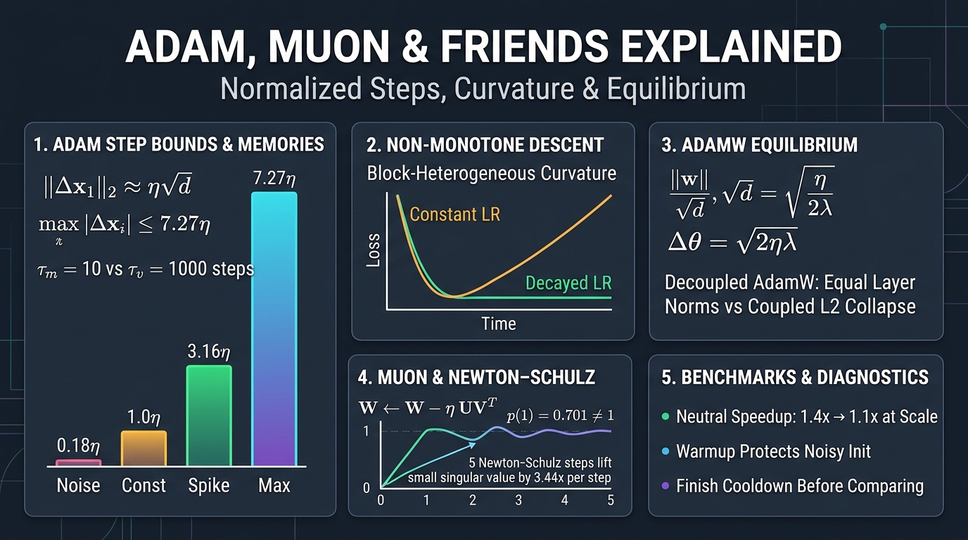
Prerequisites: the one-coordinate picture of gradient descent — a step multiplies each curvature direction by , the step is capped by the stiffest direction, the slowest sets the clock — which is §1–§2 of this package's first companion, Gradient Descent Explained. Singular values appear in §7; the one fact needed is that every matrix is a rotation, a scaling, and a rotation.
Reading path. §1–§3 are Adam, and they carry one idea three times: the normaliser makes the step's size independent of the gradient's, exactly in one case and approximately in every other, and each "approximately" has a number. §4 is why that is the right thing on a transformer-shaped problem and what it costs on a clean one. §5 is the counter-example, and what it does and does not say. §6 is weight decay, which under Adam is not a penalty but a norm. §7 is Muon, where the normalisation is per matrix instead of per coordinate. §8 is the scoreboard and how to read it. §9 is three traps.
Companion Notebook
This article pairs with the companion script worked_numbers_companions.py — NumPy only, float64, CPU-only, one seed, about sixteen seconds — which ships with this piece beside the flagship's worked_numbers.py; its B sections print every number quoted below and its A sections are the first companion's. A notebook, 01_adaptive_methods.ipynb, is built from the B sections cell for cell once the prose is final. A section number in the form §B3 beside a block names the section that printed it; the numbers are verbatim. Where a section re-computes a quantity of the flagship's script (its §12, §13, §14, §20, §21, §46, §48) it does so on its own instance under its own seed, so that the deterministic quantities agree to the printed digit and the random ones agree to sampling error.
One convention, once. Adam (Kingma & Ba 2015) keeps two exponential moving averages per coordinate, of the gradient and of its square, corrects both for starting at zero, and , and steps . The defaults are , , , and every block below uses them unless it says otherwise. Where plain momentum appears for comparison its base step is written , as in the first companion, so that always means Adam's step.
Three kinds of sentence. Every claim below is one of three things, and the text says which at the moment it is made: a theorem, true under the hypotheses stated; an identity under a model, exact for the toy it is computed on and only a guide elsewhere; or an observation at one seed, a number from one instance of one problem. The flagship grades the same claims L1–L3; here the words do the grading, and a reader who keeps the three apart will not turn a table into a theorem.
1. The first step is a sign step
Set in the formula. Then and ; and ; the update is in every coordinate — at exactly , a theorem; at the default a sign step wherever , which is every coordinate whose gradient is not within a few of zero. The first update moves each such coordinate by , in the direction of its gradient's sign, and knows nothing about the gradient's size:
§B1 Adam's first step is a sign step: ||x1 - x0||_2 is approximately eta sqrt(d) whatever the gradient's size — exactly at eps = 0, and wherever every |g_i| >> eps at the default
  d =       10: ||update||_2 / eta =      3.162   sqrt(d) =      3.162   (||g||_2 was 0.0025)
  d =     1000: ||update||_2 / eta =     31.621   sqrt(d) =     31.623   (||g||_2 was 0.0325)
  d =  1000000: ||update||_2 / eta =    999.910   sqrt(d) =   1000.000   (||g||_2 was 1.0005)
  with eps = 1e-8 the first step is -eta g / (|g| + eps), a sign step only where |g| >> eps: |step| / eta at |g| = 1, 1e-6, 1e-8, 1e-10, 0 = 1.00000, 0.99010, 0.50000, 0.00990, 0.00000; the 999.910 against 1000 above is that shortfall: each coordinate steps |g|/(|g| + eps) of a full sign step, short by eps/(|g| + eps) (about eps/|g| where |g| >> eps)
  the per-coordinate shortfall summed over the million coordinates is 94.4, and sqrt(d) - ||update||/eta = 0.090 is that sum / sqrt(d) = 0.094 to first order; the median shortfall is 1.5e-05 (|g| ~ 1e-3), so the sum is carried by the coordinates whose |g| is far below the RMS — the 842 coordinates with |g| < 1e-6 alone contribute 39.0 of it
A gradient of Euclidean length produced an update of length ; a gradient of length in a million dimensions produced one of length — the short of is : each coordinate steps of a full sign step, a shortfall of , which is at the typical here and far more on the many coordinates whose gradient happens to be near zero — the block's second line shows those carry the sum — and halves the step of a coordinate whose gradient is exactly and leaves a zero gradient where it is. At a billion parameters the first step has length . This is the oldest reason warmup exists: the first steps are sign steps, the sign of a noisy gradient at initialisation is close to random, and a small for the first few thousand steps bounds the damage while accumulates enough history to be a scale (the flagship's §5.5 has two further mechanisms). It is also the cleanest statement of what Adam is: at it is exactly sign descent, the steepest-descent direction when distance is measured by the largest coordinate rather than the Euclidean length (the flagship's §4.1), and the two averages are what make it sign descent with memory.
2. "Every coordinate moves by " — exactly when, and by how much otherwise
The intuition everyone carries about Adam is that it moves each coordinate by about per step, which is why one learning rate works across layers whose gradients differ by orders of magnitude. Here is exactly when that is true:
§B2 One coordinate under Adam: a constant gradient steps exactly eta; a gradient of constant size and alternating sign steps at most eta; a random sign steps far less
  constant g = 0.3:          |step| / eta at t = 1..6 = 1.00000, 1.00000, 1.00000, 1.00000, 1.00000, 1.00000
  g = +1, -1, +1, -1, ...:   |step| / eta at t = 1..6 = 1.00000, 0.05263, 0.33579, 0.05263, 0.20442, 0.05263   (t = 2 is 1/19 = 0.05263: m_hat = (0.09 - 0.1)/0.19, v_hat = 1)
  g = random +-1 (stationary): mean |step| / eta over steps 1000..20000 = 0.1848, max = 0.8367   (the EMA of a random sign is near zero; its RMS is 1)
While the gradient is constant — size and sign — and and the step is exactly , at every , at . That is the first line and it is a theorem. The second line keeps the magnitude constant and flips the sign: now exactly but is a weighted average of , and the step is at most and often far less — at , where the bias-corrected average is (the correction still matters at ; for large it has faded and , which is the regime every later bound is stated in). The third line is the case a training loop actually sees — a gradient whose sign is close to random from step to step — and the mean step is : the moving average of a random sign is small, its moving RMS is one, and the ratio is small. So the honest version of the intuition is: Adam's step is at most when the gradient's magnitude is steady, equal to only when its sign is too, and well below in noise.
The other direction fails as well. "At most " needed the magnitude to be steady; let it change, and the step can exceed :
§B3 Adam's per-coordinate step is not capped at eta: a quiet stretch then one unit gradient gives up to (1 - b1)/sqrt(1 - b2) = 3.16 eta; the worst history gives 7.27 eta
  b1 = 0.9, b2 = 0.999: single-spike bound (1-b1)/sqrt(1-b2) = 3.1623; supremum over all histories (Cauchy-Schwarz, t -> inf) = 7.2703
  the supremum factorises: m = (1-b1) sum_j b1^j g_(t-j), v = (1-b2) sum_j b2^j g_(t-j)^2; write b1^j = (b1^j / b2^(j/2)) b2^(j/2) and Cauchy-Schwarz gives |m|/sqrt(v) <= (1-b1)/sqrt(1-b2) x 1/sqrt(1 - b1^2/b2) = 3.1623 x 2.2991 = 7.2703, with equality iff g_(t-j) is proportional to (b1/b2)^j
      t0 quiet steps, then one unit gradient    |step| / eta at t0    geometric history g_{t-j} = (b1/b2)^j, run through Adam, |step| / eta at t = t0
         1                                          1.0000                    1.0000
        10                                          0.4844                    1.0431
       100                                          0.9758                    2.2434
      1000                                          2.5146                    5.7812
     10000                                          3.1622                    7.2701
After a long stretch of zero gradients, one unit gradient arrives: is , is , and the step is — the figure Kingma & Ba give in their §2.1 for exactly this case, reached here once the quiet stretch is long enough for the bias corrections to have faded (). And a single spike is not the worst history. Write and as the geometric sums they are, and , split each weight as , and Cauchy–Schwarz gives ; so for large , once the bias corrections have faded, , with equality exactly when . That is a bound over every gradient history, and the right-hand column runs the attaining history — a gradient that decays into the past at the rate — through Adam and reaches at (the flagship's §4.4 has the algebra with the finite- corrections). This is the shape of a rare token's embedding row: quiet for thousands of steps, then not. It is the reason gradient clipping and a non-negligible stay in the recipe, and the reason " is the per-coordinate step" is a trust-region intuition and not a bound. The bound is .
3. The two memories
The whole of §2 is a statement about two time constants. forgets at the rate : after ten steps it has absorbed of a new gradient, after a hundred all of it. forgets at the rate : after a hundred steps it has absorbed under of a new scale, after a thousand :
§B9 The two memories: how much of a new gradient scale v has absorbed after t steps, 1 - b2^t, and the effective learning rate the momentum gives a constant gradient, 1/(1 - b1)
        t      1 - 0.999^t (share of a new scale in v)     1 - 0.9^t (share in m)
        1              0.0010                                  0.1000
       10              0.0100                                  0.6513
      100              0.0952                                  1.0000
     1000              0.6323                                  1.0000
     3000              0.9503                                  1.0000
    10000              1.0000                                  1.0000
  time constant of v: 1/(1 - b2) = 1000 steps; of m: 1/(1 - b1) = 10 steps; a constant gradient's effective step under plain momentum (no normaliser) is alpha/(1 - beta) = 10 alpha at beta = 0.9
So is a ten-step average divided by a thousand-step RMS, and every number in §2 is a consequence of that mismatch: the spike exceeds because has already caught the new gradient while still remembers the old quiet; the random sign steps below because a ten-step average of is small while the thousand-step RMS is one. is the knob that sets how long the scale is trusted, and it is a knob with a wrong setting (§9.1), not merely a noisy one. The last line is the one fact about momentum that is pure algebra and that every reader should carry: without a normaliser, a constant gradient's effective step under momentum is , ten times at . Adam's normaliser removes exactly that factor — on a constant gradient — which is one more way to say that Adam's and SGD-with-momentum's are not the same kind of number.
4. The problem Adam is right for, and the one it is not
Why does Adam beat SGD on transformers by a margin it does not show on convolutional nets? The explanation with the most controlled evidence is about curvature, and the smallest model of it is a quadratic with blocks:
§B4 Block heterogeneity: a 4-block quadratic (25 coordinates each, curvatures 1, 10, 100, 1000) — one learning rate for all against one per block, and Adam at a constant step
  f(x0) = 15858.56; GD with the one safe step 1/L (L = 1000): 10529 iterations to f < 1e-8 (the curvature-1 block contracts by (1 - 1/1000)^2 per step)
  per-block step 1/L_block: f after 1 step = 6.9e-30  (each block is a scalar quadratic; a diagonal preconditioner is exact)
  Adam eta = 0.1   constant        : f at t = 100, 500, 1000, 2000, 3000 = 2.746e-01, 2.151e-19, 2.826e-42, 1.178e-04, 4.042e-03;  max f over t in [1000, 3000] = 1.482e+00
  Adam eta = 0.01  constant        : f at t = 100, 500, 1000, 2000, 3000 = 3.133e+03, 1.151e+00, 2.752e-08, 1.904e-39, 1.651e-09;  max f over t in [1000, 3000] = 1.631e-02
  Adam eta = 0.1   decayed x0.995/step: f at t = 100, 500, 1000, 2000, 3000 = 1.740e-01, 8.172e-20, 1.907e-28, 3.233e-29, 3.164e-29;  max f over t in [1000, 3000] = 1.907e-28
  at a constant step Adam is not monotone even on a noiseless quadratic: once the gradient has been tiny for ~1/(1-b2) steps v forgets the old scale, m/sqrt(v) grows back toward one and a step of ~eta per coordinate kicks the iterate out of the minimum it had reached; a decaying step removes the re-excitation
Four blocks of twenty-five coordinates with curvatures , , , . One learning rate for everything must be for the stiffest block, and then the softest block converges at : ten and a half thousand steps. One learning rate per block, set from the block's known curvature, solves the whole problem in one step, because each block is a scalar quadratic and a diagonal preconditioner built from the Hessian is exact on a diagonal Hessian. That row is the ideal benchmark, not Adam: Adam estimates a per-coordinate gradient scale from its moments, which tracks the curvature only in the sense that a stiff block's gradients are larger, and it needs the memory of §3 to form the estimate — the three Adam rows are what the estimate actually does. Zhang et al. (2024) measured the Hessian of transformers blockwise — embedding, each attention projection, each MLP matrix — and found exactly this picture: block spectra differing by orders of magnitude, where a CNN's do not; SGD on par with Adam without the heterogeneity and worse with it. On the quadratic the claim is a theorem; as the explanation for transformers it is the best-evidenced of three mechanisms that are not exclusive of each other (the flagship's §4.4 grades all three).
Now read the three Adam rows, because they show the cost of the same normaliser on a clean problem. At Adam is at by step and by step — far faster than gradient descent could be — and then at step the loss is , and the largest value it took between steps and is , above where it was at step . Adam at a constant step is not monotone, even here, with no noise and a convex quadratic.
The mechanism is §3: once the gradient has been tiny for about steps, has forgotten the old scale; drifts back toward one; and the step, which is again per coordinate, kicks the iterate out of a minimum it had reached to forty digits. At the same thing happens later and smaller. A decaying step removes the re-excitation entirely — the third row sits at and stays. This is one seeded instance, not a theorem: it shows that a constant-step Adam near a minimum can re-excite itself and that the mechanism is the memory. Whether the re-excitation settles into a periodic cycle, and at what size, depends on the problem and the step, and we claim no general limit-cycle result. What the instance does establish is that monotone descent is not a property of the method, and that the schedule is not optional.
5. The counter-example, and what it does and does not say
Kingma & Ba's convergence proof had a gap, and Reddi, Kale & Kumar (2018) closed it in the wrong direction: there is a convex problem on which Adam does not converge. Online linear losses on : the gradient is every third round and otherwise, with , so the loss over one period is and the best point is .
§B5 Reddi, Kale & Kumar (2018): online linear losses on [-1, 1], gradient C every third round and -1 otherwise — Adam drifts to the wrong end, AMSGrad does not
  C = 3.0, beta2 = 1/(1+C^2) = 0.100, beta1 = 0, eta_t = 0.1/sqrt(t) (the setting of their Theorem 1): after 5000 rounds Adam sits at x = +1.000 (average regret +0.6536);  AMSGrad at x = -1.000 (average regret +0.0381)
  same sequence with the default first-moment coefficient beta1 = 0.9 and bias correction, beta2 kept at 0.1 (not the full defaults): Adam sits at x = -1.000 (average regret +0.0098) — the momentum averages the three gradients to (C - 2)/3 > 0 before the normaliser sees them, and the drift reverses; Theorem 2 of the paper builds a different sequence for beta1 > 0
  same sequence at the full defaults (beta1, beta2) = (0.9, 0.999) with bias correction: Adam sits at x = -1.000 (average regret +0.0140); the displayed three-period example uses beta2 = 0.1 — the theorem is not restricted to that value, but the sequence that defeats a long beta2 is a different and longer one
  the sum of losses over one period of 3 is (C - 2) x = 1.0 x, minimised at x = -1; with beta1 = 0 the step after the C-gradient is small (v just jumped) and after each -1 gradient it is large: net drift is toward +1
The mechanism is §3 once more, with a short : the large gradient inflates , so the step that follows it is small; the two gradients of that follow let decay, so their steps are large; the net motion per period is toward , the wrong end, and Adam sits there with a regret that grows linearly. AMSGrad — replace by its running maximum, so the effective step never increases — converges to . The theorem is real: Adam's regret can be on a convex problem for any constant .
Now the second line, which the paper's readers often miss. Run the same gradient sequence through Adam with the default first-moment coefficient (bias-corrected), keeping , and it goes to , the right end, with an average regret of ; at the full defaults it goes to as well, regret : the momentum averages the three gradients to before the normaliser sees them, and the drift reverses. The theorem for is true, but it needs a different sequence (their Theorem 2 builds it), and the sequence above is the one. Two honest conclusions. The failure is narrower than the theorem reads: the displayed three-period example uses and an adversarial order — the theorem is not restricted to that , but the sequence that defeats a long one is a different and longer construction — and nobody runs a of . And it is not empty: the paper's stochastic version needs a rare large gradient against many small ones — the shape of a rare token's gradient, §2 again — and that one is not exotic. The AMSGrad fix ships as an off-by-default flag in every framework; what practice does instead is run close to one, which is precisely the hypothesis the positive convergence results need (Défossez et al. 2022).
6. Weight decay under Adam is a norm, not a penalty
For a weight followed by a normalisation layer — which is most of a modern network — the function does not depend on , and an penalty "regularises" nothing about the function. What it does is set the norm, and through the norm, the angle by which each update turns the weight. The computation is the AR(1) of the first companion's §5 in another costume: under AdamW's decoupled update , with an update of unit RMS per coordinate that is uncorrelated with , the squared norm obeys , whose fixed point is , and the angular step is then :
§B6 Weight decay under Adam-style updates is an equilibrium: decoupled (AdamW) settles ||w||/sqrt(d) at sqrt(eta/(2 lambda)) and the angular step at sqrt(2 eta lambda); coupled L2 does not
  d = 1000, eta = 0.01, lambda = 0.1: equilibrium ||w||/sqrt(d) = sqrt(eta/(2 lambda)) = 0.2236, angular step sqrt(2 eta lambda) = 0.0447 rad, timescale 1/(eta lambda) = 1000 steps
  decoupled:  t      ||w||/sqrt(d)    angular step this update (rad)
                 1       2.9969           0.0033
               100       2.7144           0.0037
              1000       1.1243           0.0087
              3000       0.2757           0.0364
             10000       0.2273           0.0440
  two layers under Adam's normaliser: gradient noise RMS 1 (first half) and 0.01 (second half); ||w||/sqrt(d/2) per half at t = 1000, 3000, 10000
    decoupled (AdamW)                        : t=1000: 1.1178 / 1.1205   t=3000: 0.2639 / 0.2491   t=10000: 0.2123 / 0.2213
    coupled L2 (lambda w inside the gradient): t=1000: 1.1470 / 0.0077   t=3000: 0.2666 / 0.0133   t=10000: 0.2076 / 0.0218
  why the two-layer rows sit near 0.2226 and NOT at 0.230 x 0.2236 = 0.0515: Adam's update is a momentum average of the normalised noise, so its one-step RMS is only about sqrt((1-b1)/(1+b1)) = 0.2294 of the noise's (0.230 measured), but successive updates are correlated and the AR(1) recursion sums that correlation
  scalar proxy m_t = b1 m_(t-1) + (1-b1) g_t, w_(t+1) = (1 - eta lambda) w_t - eta m_t, unit Gaussian g: exact stationary RMS of w = eta sqrt( (1-b1)/(1+b1) * (1 + a b1) / ((1 - a^2)(1 - a b1)) ) = 0.2226 with a = 1 - eta lambda = 0.999; simulated over 1000 coordinates at t = 20000: 0.2227; the uncorrelated-noise formula sqrt(eta/(2 lambda)) = 0.2236 lands within 0.5% of it because the correlation factor (1 + a b1)/(1 - a b1) = 18.82 almost exactly cancels the variance factor (1-b1)/(1+b1) = 0.0526
  (so the same-norm-in-both-layers result stands — the normaliser hands both layers unit-RMS noise before the momentum — but it is a statement about a correlated AR(1), not 'the update RMS times the formula'; the coupled form's second layer, where lambda w dominates the gradient, is driven to a different norm by a decay the normaliser has rescaled)
Started at an RMS of per coordinate, the norm takes about steps to decay and settles at against the predicted ; the angular step settles at radians against , about per update, independent of the gradient's scale and of the start. The two consequences are the ones the flagship's §5.6 grades: and are not two knobs — their product sets the rotation rate and their ratio sets the norm, and the norm is invisible to the function; and the first steps are a transient in the norm, which is one reason warmup and weight decay interact.
The second block is why AdamW (Loshchilov & Hutter 2019) is not Adam with an term. Take two "layers" whose gradient noise differs by a factor of a hundred. Under the decoupled form both settle at the same norm — and , against from the computation below — because the normaliser makes the update's statistics the same in both layers and the decay is applied outside it. Under the coupled form, where is added to the gradient before the normaliser, the second layer collapses to by step : there the decay term dominates the gradient, the normaliser rescales it to a unit-sized step, and the layer is driven toward zero by a force that has nothing to do with 's nominal value. The coupled form gives every layer a different effective decay set by that layer's gradient scale; the decoupled form gives every layer the same equilibrium. That is the whole of the "AdamW is better" claim at the level of algebra; whether it generalises better is a measurement, and the flagship labels it one.
One correction to the first paragraph's recipe, because it is the kind of shortcut this piece exists to catch. The formula assumed an update that is uncorrelated from step to step. Adam's update is a momentum average of the normalised noise, so its one-step RMS is only — and the tempting fix, "multiply the formula by that RMS", gives , which the table refutes. The reason is temporal correlation: successive updates share the same , and the AR(1) recursion for picks up the cross term between the weight and the update. For the scalar proxy , with unit Gaussian , the exact stationary variance is with : the variance factor and the correlation factor nearly cancel, and the RMS is , within of the uncorrelated formula's — the block's last lines compute it and simulate it. So the two-layer rows illustrate a scale-independent equilibrium whose value the correlated AR(1) predicts; the uncorrelated formula lands nearby at these constants by that near-cancellation, and it is the correlated computation, not the instantaneous RMS, that says why.
7. Muon: normalise the matrix, not the coordinate
A network's parameters are mostly matrices, and a per-coordinate normaliser treats a matrix as a long vector. Muon (Jordan et al. 2024) does not: it takes the momentum of a weight matrix's gradient and replaces it by its polar factor — the matrix with the same singular directions and every singular value set to one — and steps . That is the steepest-descent direction when distance is measured by the spectral norm (the flagship's §4.5; Bernstein & Newhouse 2024 is the paper that puts Adam, Shampoo and Muon in one family by the norm each one descends under). Computing by an SVD each step is too expensive; Muon instead runs five steps of a Newton–Schulz iteration, with , a polynomial tuned to lift small singular values fast — not, as the block shows, to converge to one. Here is what five steps do to an gradient whose smallest singular value we forced to be tiny:
§B7 Newton-Schulz orthogonalisation (Muon's coefficients 3.4445, -4.7750, 2.0315), five steps on an 8 x 4 Gaussian gradient with one singular value forced small
  singular values after Frobenius scaling: [0.8093 0.4446 0.3839 0.0008]
  NS step 1: singular values -> [1.1471 1.0691 0.9619 0.0028]
  NS step 2: singular values -> [0.7787 0.7364 0.685  0.0096]
  NS step 3: singular values -> [1.1311 1.0696 1.0093 0.0331]
  NS step 4: singular values -> [0.7472 0.6948 0.6852 0.1137]
  NS step 5: singular values -> [1.1309 1.1206 1.0548 0.3848]
  after 5 steps: ||X||_2 = 1.1309 (exact polar factor: 1), ||X||_F = 1.9482 (exact polar factor: sqrt(min(m, n)) = 2.0000); the five-step update is 2.6% short of the ideal Frobenius norm
  near zero p(sigma) = 3.4445 sigma - 4.775 sigma^3 + 2.0315 sigma^5 ~ 3.44 sigma: a value of 8.09e-04 needs about log(1/sigma)/log(3.44) = 5.8 steps to reach the band where the healthy values live
  p(1) = 0.7010: 1 is NOT a fixed point of these coefficients (the classical Newton-Schulz cubic 1.5 s - 0.5 s^3 has p(1) = 1, p'(1) = 0); the positive fixed points are s = 0.8680 and 1.2637 with |p'(s)| = 1.58 and 6.47, both > 1 and so both unstable — the iteration never converges to 1, it oscillates in a band (rows above), a trade the coefficients make for the x3.44 lift near zero
  per-entry RMS of the exact polar factor on m x n = 8 x 4: sqrt(min/(m n)) = 1/sqrt(max(m, n)) = 0.3536 (measured 0.3536); Moonshot's 0.2 sqrt(max(m, n)) = 0.5657 rescales it to RMS 0.200, AdamW's typical per-coordinate update RMS
Three things to read. First, the three healthy singular values, which started at , , , end at , , — near one, not at one, and on this instance all above it. That is not a convergence cut short: these coefficients have no fixed point at one. Substitute and ; the polynomial's positive fixed points are and , both unstable ( and ), so the iteration oscillates in a band — watch the rows alternate between about and — rather than settling. The classical Newton–Schulz cubic does have and and converges quadratically; Muon's authors traded that for a steeper slope at zero, deliberately, because five steps of a fast lift are worth more to them than an exact orthogonalisation. Second, the tiny one: , a factor of per step, because near zero the polynomial is . A singular value of needs about six steps of that lift to reach the band where the healthy values live, and gets five, so it ends at . Third, the measured consequence: the exact polar factor has spectral norm and Frobenius norm ; the five-step output has and , so the actual update is over in spectral norm and short in Frobenius norm on this matrix (the flagship's instance is over and short — the gap depends on the singular-value spread, which is the point: here three of four values are healthy, there two of four were small). Every statement of the form "Muon's update has size exactly " is a statement about , true for the ideal and approximate for what the code does.
The last line is why one learning rate can serve Adam and Muon in the same run. The exact polar factor's per-entry RMS is — on — and AdamW's per-coordinate update RMS is typically around ; Moonshot's recipe (Liu et al. 2025) multiplies the Muon update by so that both have RMS . What that matching buys is one thing exactly: the weight-decay equilibrium of §6 becomes transferable — the same and give both methods the same equilibrium norm and the same predicted rotation rate. What it does not buy is an identical step: the orthogonalised update spends its length equally across singular directions where Adam's spends it per coordinate, so the effective step per direction differs between the two methods, and a learning-rate sweep on each is sweeping a different thing. And the shared rotation rate is a prediction under §6's idealisation — a unit-RMS update uncorrelated with — so the actual angular rates of Muon and AdamW in a run are a measurement to take, not a number to assume.
Does the direction help? On a problem whose difficulty is in the input directions rather than the coordinates, it should, and here is an illustration — an ill-conditioned matrix regression, rotated so that the stiffness is not aligned with the coordinates Adam normalises:
§B8 Four methods on an ill-conditioned matrix regression (16 x 32 weights, input covariance condition number 1e4), each at the best step from a grid, step decayed x0.998 per iteration, input rotated so the stiffness is not axis-aligned — an illustration, not a theorem
  loss at W = 0: 3.3805e+01; largest eigenvalue of the input covariance 0.9394, smallest 6.65e-05
  GD                                   best step  1.9500: t=100: 6.083e-02  t=1000: 1.112e-02  t=2000: 9.715e-03
  GD + momentum 0.9                    best step  3.5000: t=100: 3.999e-03  t=1000: 1.476e-04  t=2000: 1.051e-04
  Adam                                 best step  0.3000: t=100: 2.654e-02  t=1000: 1.123e-03  t=2000: 6.301e-04
  Muon-like (orth of momentum 0.9)     best step  0.1000: t=100: 1.154e-01  t=1000: 3.357e-04  t=2000: 6.525e-06
  the problem was built to be ill-conditioned in exactly the way a per-direction step fixes; a fixed-length update in every singular direction overshoots the easy ones early and wins late
  the same instance unrotated (Qrot^T applied, no new draw; the stiffness is axis-aligned) — the pilot the prose compares against:
    GD                                   best step  1.9500: t=100: 6.889e-02  t=1000: 1.426e-02  t=2000: 1.243e-02
    GD + momentum 0.9                    best step  3.5000: t=100: 3.748e-03  t=1000: 9.864e-05  t=2000: 6.816e-05
    Adam                                 best step  0.3000: t=100: 2.826e-04  t=1000: 6.072e-31  t=2000: 5.417e-31
    Muon-like (orth of momentum 0.9)     best step  0.1000: t=100: 1.059e-01  t=1000: 2.497e-04  t=2000: 6.236e-06
    unrotated, Adam's t=2000 loss is 25.1 orders of magnitude below the best of the other three; rotated, it is an ordinary method
  but axis-aligned is not the same as exactly preconditioned: H = diag(1, 100), x0 = (2, 1), gradient (2, 100); the exact Newton step is (-2, -1) and Adam's first eps-free step is eta x (-1, -1) — component ratios 2:1 against 1:1, so no scalar eta makes them equal; 1/sqrt(v_hat) is a gradient scale, not the inverse Hessian, even on a diagonal quadratic
The orthogonalised update is the worst of the four at a hundred steps — a fixed-length step in every singular direction overshoots the easy ones before the step has decayed — and the best by a factor of sixteen over momentum and a hundred over Adam at two thousand, because the -scaled input directions get the same step as the -scaled ones. Note what the rotation did to Adam. On the unrotated instance — the block's second table, the same draw with the rotation undone — the curvature directions line up with the parameter coordinates, a per-coordinate scale is the right shape, and Adam is at by a thousand steps, twenty-five orders of magnitude below the best of the other three at two thousand; rotate the inputs so the stiffness is spread across coordinates and Adam is an ordinary method again. The right shape is not exact preconditioning: Adam's is a gradient scale, not the inverse Hessian, even on a diagonal quadratic — on from the Newton step is and Adam's first -free step is , and no scalar makes those equal (the block's last line). The exact one-step solver on a diagonal problem is §4's per-block row, built from the Hessian; Adam's coordinate-wise normalisation estimates that shape from gradient moments, which is very effective when the problem is diagonal and no better than momentum when it is not. This block is labelled an illustration because it is one: the problem was built to be ill-conditioned in exactly the way the spectral direction fixes, and the theorems that exist for Muon are stationarity rates under spectral-norm smoothness (the flagship's §4.5 lists them), not speedup theorems for a transformer.
8. The scoreboard, and how to read one number on it
The claim that sells Muon is " the compute efficiency of AdamW". Here is how to grade it, and the flagship's §4.6 does so for the whole 2025–26 field. Liu et al. (2025) measured it in their own scaling-law runs, which makes it a vendor's number — not wrong, but to be quoted with that label. The neutral benchmark, AlgoPerf (Dahl et al. 2023; Kasimbeg et al. 2025), had Distributed Shampoo win its tuned track by about over the baseline and schedule-free AdamW win its self-tuning track by about . Wen et al. (2025) ran ten optimizers at –B parameters with equal tuning and found the matrix methods' speedup over a tuned AdamW to be at B shrinking to about at B, and named the two traps that inflate a comparison: unequal tuning, and comparing runs before the learning-rate decay has finished — which, after §4 and the first companion's §5, you can now see is comparing one run's floor to another's transient. Khona et al. (2026) report SOAP and Muon ahead of AdamW at multi-billion scale and stable at batch sizes where AdamW degrades; that is a vendor's run too, and a recent one.
So the practitioner's reading: the direction is a theorem (steepest descent under the spectral norm), the approximation to it is measured (§7), the speedup is a measurement about a model family at a scale, it shrinks with scale in the one neutral multi-scale study, and the single most valuable thing an optimizer comparison can do is finish the cooldown before it reads the loss.
9. Where intuition breaks, and what to do instead (deeper reading)
9.1 — " is just smoothing; any value near one is fine." §5. A short is wrong, not noisy — it is the hypothesis of the counter-example — and a long one is the hypothesis of the convergence proofs. The symptom of a that is too short for your gradient statistics is a loss that spikes on rare inputs; the fix is a longer , the AMSGrad flag, or clipping.
9.2 — "Warmup is always needed." It is needed for the reasons it exists, and not otherwise:
§B10 Warmup on the 4-block quadratic from a far start (RMS 10): Adam at eta = 0.1 with no warmup against a 100-step linear warmup
  no warmup           : f at t = 10, 50, 100, 200, 500 = 1.358e+06, 7.132e+05, 3.133e+05, 5.974e+04, 1.151e+02
  linear warmup 100 st.: f at t = 10, 50, 100, 200, 500 = 1.573e+06, 1.304e+06, 7.317e+05, 1.606e+05, 9.697e+02
  f(x0) = 1.586e+06, ||x0||_2 = 99.2; the first Adam step moves every coordinate by eta, ||x1 - x0||_2 = eta sqrt(d) = 1.0, whatever the gradient — harmless here, because this quadratic has no noise and no sharpening for warmup to protect against; the gain warmup shows in a transformer is a measurement about the transformer, not a theorem about descent
On a noiseless quadratic from a far start, warmup only costs: eight times the loss at step . The sign step of §1 is harmless when the gradient's sign is right, and here it is; warmup protects against a noisy sign at initialisation, against a sharpening landscape, and against instabilities that grow with scale (the flagship's §5.5), none of which this problem has. The point is not that warmup is useless — it is close to free at pretraining scale and the divergence it prevents is not — but that its benefit is a measurement about the model, and a reader who sees no gain from it on a clean problem has not found a bug.
9.3 — "Adam's loss is flat, so it converged." Two floors are possible, and they need different fixes. Under noise, the floor is the first companion's §5 and the fix is a cooldown. With no noise, §4: a constant-step Adam near a minimum can re-excite itself as forgets, on the timescale and at a size of order per coordinate — an observation on the block quadratic, not a theorem — and the fix is the same cooldown for a different reason. Either way, flat is not converged, and a decayed step tells you which floor you were on by how far it drops.
What to take away
- Adam's first step is a sign step of length , whatever the gradient — exactly at , to within per coordinate at the default. at a billion parameters; the oldest reason for warmup; at Adam is sign descent.
- "Every coordinate moves by " is a theorem for a constant gradient, an upper bound for a constant magnitude, and false in general. at the second step of an alternating sign; on average in noise; after a quiet stretch; at the supremum, attained by a history a run can produce. The bound is , and clipping and are in the recipe because of it.
- The two memories are ten steps and a thousand steps. Every excess and every shortfall in point 2 is the ten-step average disagreeing with the thousand-step RMS; is how long the scale is trusted.
- A per-coordinate scale is the right shape on a diagonal problem — exact when built from the Hessian, an estimate when Adam builds it from gradient moments — and ordinary on a rotated one. One step against on the block quadratic; the transformer's blockwise Hessian is the measured reason Adam wins there. At a constant step Adam is not monotone even on a noiseless quadratic — at step , somewhere before step , on this instance — and a decayed step removes it.
- The displayed Reddi sequence is the , short- construction; the theorem is broader — any constant fails on some sequence — but with the default , at or at the full defaults, the displayed sequence converges and a different one is needed. Narrower than it reads, not empty: a rare large gradient against many small ones is the stochastic version, and that is what a rare token looks like.
- Weight decay under AdamW sets a norm, , and an angular rate, , the same in every layer. Measured and against and ; under momentum the update is correlated in time and the exact AR(1) gives , not the update RMS times the formula. Coupled gives each layer a decay rescaled by its own gradient: in one layer and in another at the same .
- Muon's direction is a theorem; its five-step Newton–Schulz is an approximation whose error you can measure. over in spectral norm and short in Frobenius norm here, and on the flagship's instance; the coefficients have no fixed point at one () and oscillate in a band by design; a small singular value grows by per step and needs six to reach that band. The is a vendor's measurement; the neutral multi-scale study has shrinking to ; finish the cooldown before you compare.
Where to go next
The companion script worked_numbers_companions.py prints every number above in its B sections; its A sections carry the first companion, Gradient Descent Explained, which is where the step ceiling, the condition number, the noise floor and the schedule question that this piece keeps pointing back to are built from one coordinate up.
This package's flagship, The Optimization Domain, takes each section here one level down: §4.1 for steepest descent under a norm, which is the one idea that makes Adam, Shampoo and Muon one family; §4.4 for Adam with the Cauchy–Schwarz bound, the counter-example's theorem and the three mechanisms behind "Adam wins on transformers", each graded; §4.5 for Shampoo, SOAP and Muon with the stationarity theorems that exist; §4.6 for the 2025–26 scoreboard quoted from the neutral benchmarks; §5.5–§5.6 for warmup and the weight-decay equilibrium at full size; and §11 for the assumption map that says, claim by claim, which of these is a theorem and under what hypothesis. Our Information Domain is where mirror descent and the natural gradient — the two other geometries of the step — come from.
For deeper reading: Kingma & Ba (2015) is short and worth reading in the original, §2.1 in particular; Reddi, Kale & Kumar (2018) for the counter-example and AMSGrad; Loshchilov & Hutter (2019) for the decoupling; Bernstein & Newhouse (2024), Old Optimizer, New Norm, for the one-family view; Jordan et al. (2024) for Muon as it was first written up, and Liu et al. (2025) for the recipe that made it run at scale; Kasimbeg et al. (2025) and Wen et al. (2025) for the two comparisons that controlled for tuning; and Kosson, Messmer & Jaggi (2024) for the rotational-equilibrium view of weight decay that §6 is the smallest instance of.
We build agent systems and practitioner tooling at Artifocial — see our apps, including Alarmly.