Information Theory Explained: Entropy, Cross-Entropy, and the Loss You Already Use
Information theory for practitioners who need it for machine learning: what a bit actually measures, why minimising cross-entropy is minimising KL divergence, the floor label smoothing installs under your loss (and which smoothing convention your framework uses), and why a mutual-information estimate is a measurement with a sign that depends on the regime, not a number.
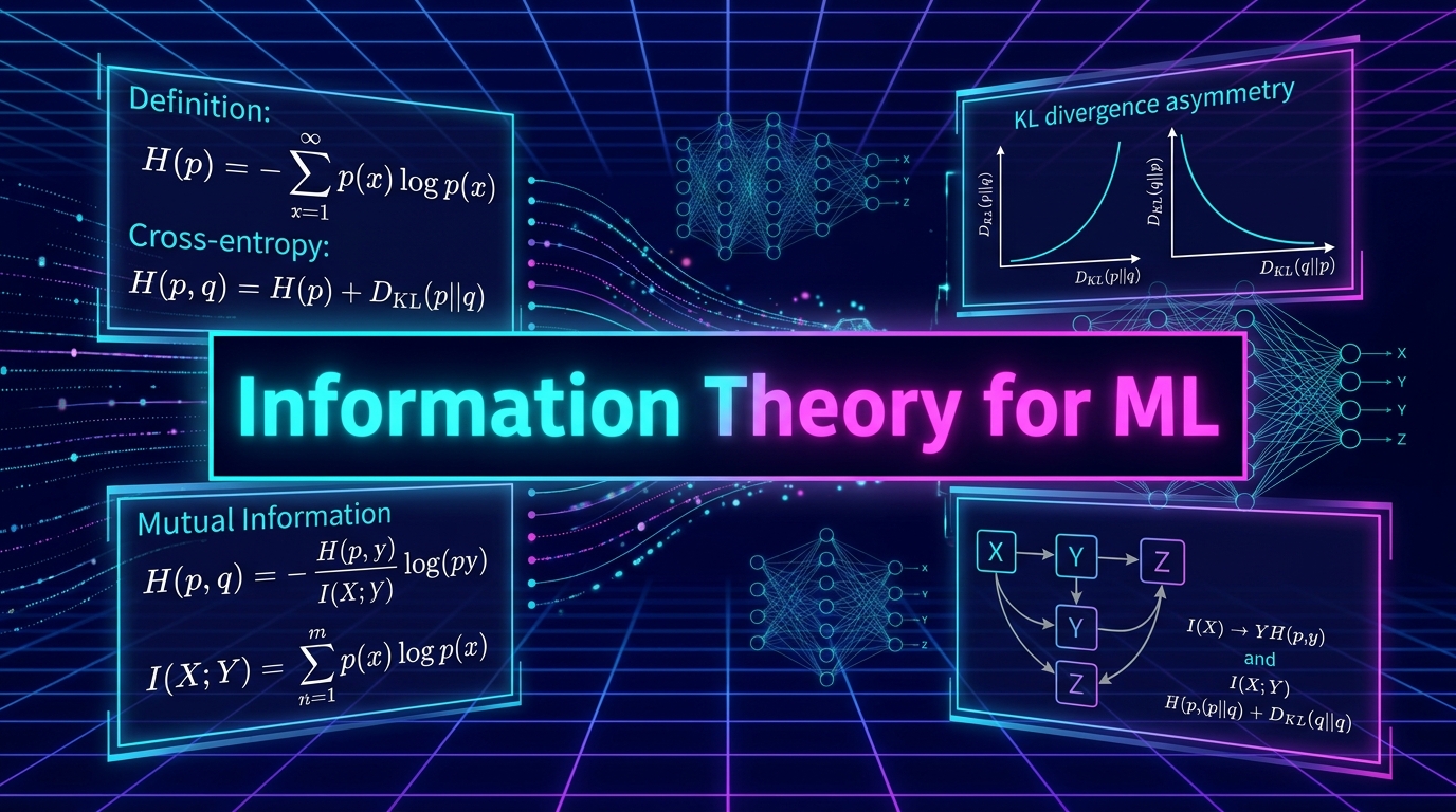
Prerequisites: comfort with probability distributions and logarithms; nothing else. If you want the machinery before the intuition, start at §2 and come back to §1.
Reading path. If this is your first pass, the core is §1–§5, and it carries four ideas: what a bit means, why cross-entropy is entropy plus KL, why label smoothing installs a floor under your loss, and why information cannot be recovered once it is gone. §6 (the estimator's bias) and §7 (the two numerical traps) are deeper reading for the day you start measuring these quantities yourself; nothing in §1–§5 depends on them.
Companion Notebook
This article pairs with 00_information_theory_from_scratch.ipynb — pure NumPy and Matplotlib, CPU-only, every figure inline, and the two small networks' backward passes written out by hand and checked against finite differences. It carries the same material in runnable form: entropy and cross-entropy from their definitions, the decomposition identity verified over 20,000 random pairs, a maximum-entropy experiment over 200,000 random distributions, the label-smoothing floor tabulated across vocabulary sizes under both conventions in common use, mutual information on a binary symmetric channel checked against its closed form, the data-processing inequality tested on 5,000 random Markov chains, and the plug-in estimator's bias measured in both directions — against a ground truth that is exactly zero, where it reads high, and against a perfectly dependent pair, where it reads low.
Every table and printed block quoted below is copied from that notebook's output — Python 3.14.5, NumPy 2.5.3, seed 20260921 fixed in the first cell, so a re-execution in that environment reproduces every one of them; a few values in the prose are derived from those outputs or from the closed forms on the page rather than printed by the notebook, and are marked where they appear. The notebook's first cell prints the environment and the reproducibility scope; nothing quoted here depends on a trained network, which is the one part of the companion notebook that does not travel across platforms (the bottleneck piece says why). Two common mistakes are taken apart below, each with its counter-example: a smoothing-floor table that does not say which convention produced it, and the rule that a mutual-information estimate is always an upper bound.
Units, once. We write and say bits unless a line says otherwise. A cross-entropy loss as a framework computes it is in nats per token under mean reduction, so the floor tables below print both; every printed number carries its unit, and mixing the two inside one subtraction is the commonest way to get a wrong floor out of a right table.
1. What a bit actually measures
Most explanations of information theory begin with a definition and hope the intuition arrives later. Let us go the other way, because the intuition is genuinely simple and it makes the formula obvious rather than arbitrary.
Suppose I pick a number from 1 to 8 and you have to find it by asking yes/no questions. If you ask well — "is it above 4?", then "is it above 6?", then "is it 8?" — you always need exactly three questions. Eight possibilities, three questions, and .
That is the whole idea. The information content of an outcome is the number of yes/no questions needed to pin it down. And since , the number of questions for equally likely options is .
Now make it unequal. If I am picking a letter from English text, "e" is common and "z" is rare. Learning that the letter is "z" is more informative than learning it is "e", because "z" eliminates far more possibilities. So the surprise of an outcome should grow as its probability shrinks. The quantity that does this, and does it in a way that makes independent surprises add up, is:
The logarithm is not a stylistic choice. It is forced by one requirement: if two things are independent, their surprises should add. The probability of two independent events multiplies, and the only function that turns multiplication into addition is the logarithm. Everything else in this article follows from that one constraint.
Entropy is just the average surprise, weighted by how often each outcome actually happens:
Read it as: on average, how many yes/no questions will I need? From the notebook:
H(uniform over 8)   = 3.000000 bits   (exact: log2(8) = 3)
H(point mass)       = 0.000000 bits   (exact: 0)
H(dyadic skewed)    = 1.875000 bits   (exact: 1.875)
Three bits for eight equally likely options — the question game, confirmed. Zero bits for an outcome that is certain, because there is nothing to ask. And 1.875 bits for a skewed distribution, which is less than 3: when some outcomes are more likely than others, you can be cleverer about your questions, asking about the likely ones first. That is exactly what a compression algorithm does.
One honest footnote to the question game, because the slogan is slightly stronger than the theorem. Entropy is the expected number of questions only when every probability is a power of two, as in the 1.875-bit example above (that is what "dyadic" means). For a general distribution the best question scheme — a Huffman code — needs on average questions with , and the gap can be most of a bit: a coin with has entropy 0.469 bits, but you still have to ask one whole question to learn one toss. The entropy is reached per symbol only when you ask about long blocks of tosses at once, which is Shannon's source-coding theorem. So read as the number of questions in the limit, and treat as what a single draw can cost you. And that per-symbol limit is when the source produces independent draws from the same distribution. When successive symbols are correlated, the limit is the entropy rate, , which can be smaller — draw one fair bit and repeat it forever, : every symbol has entropy 1 bit, the whole sequence holds one bit of uncertainty, and the entropy rate is zero. Text is the correlated case, so its lossless-compression limit is governed by an entropy rate. A language model's held-out per-token loss measures the model's cross-entropy rate — its codelength per token on that text — which exceeds the source's entropy rate whenever the model is imperfect; it is a statement about a rate, not about any one token's entropy, and §3.1 keeps the two rates apart.
1.1 Uniform really is the maximum
It is standard to assert that the uniform distribution has the highest entropy. The proof is two lines — by Jensen's inequality, since is concave, with equality only when is uniform on all outcomes — and it is still worth watching the inequality fail to be beaten, as long as you read the picture as a picture and not as the argument. The notebook samples 200,000 random distributions over eight outcomes:
Maximum-entropy check over 200,000 random distributions on 8 outcomes:
  max H found = 2.979046 bits   vs uniform's 3.000000
  exceeded uniform in 0 of 200000 draws
Two hundred thousand attempts, closest approach 2.979, never exceeded. Maximum uncertainty means every option equally likely — which is why "maximum entropy" is the formal way of saying "I am assuming as little as possible."
1.2 The number worth memorising
One example does more work than any other for building intuition:
A fair coin is exactly 1 bit. A coin with is 0.4690 bits — so nine-to-one odds have already destroyed more than half the uncertainty of a fair coin.
Sit with that for a moment, because it is not what most people guess. A 90/10 coin still feels fairly uncertain — it comes up tails one time in ten, which you would notice. But in information terms more than half the uncertainty is already gone.
Entropy falls off fast as a distribution concentrates. This is why the gap between a model that is 90% confident and one that is 99% confident matters so much more than the 9-percentage-point difference suggests, and it is the first hint that confident-but-wrong is a much more expensive failure than unconfident-and-wrong.
2. Cross-entropy: what it costs to be wrong
Entropy assumes you know the true distribution . In practice you have a model , and is not . Cross-entropy is what your code costs when you build it for but the data actually comes from :
The data arrives according to — that is the weight out front. The number of questions you ask is designed for — that is the logarithm. You pay 's frequencies at 's prices.
The concrete version: you build a compression scheme expecting mostly the letter "e", so you give "e" a short code. If the text is actually full of "z", you are spending long codes constantly. Your file is bigger than it needed to be. Cross-entropy is that bigger size.
KL divergence is the size of the mistake — the excess over what a perfect code would have cost:
And these three quantities are related by an identity that is the single most useful line in this article:
In words: the cost of using the wrong model = the cost that was unavoidable + the cost of being wrong.
This is an algebraic identity, not an approximation, so the right way to check it numerically is to confirm it holds to floating-point precision. Over 20,000 random pairs:
(a) max |H(p,q) - [H(p) + KL(p||q)]| over 20,000 random pairs = 8.882e-168.882e-16 is machine epsilon territory. Be clear about what that check is: it confirms that our implementation agrees with an algebraic identity whose proof is one line (expand the log of a ratio), and nothing else — it is not evidence for the identity, and it does not vouch for any other experiment in the notebook. The identity is exact; the check is a software test.
Two further properties, also measured rather than asserted:
(b) min KL over 100,000 random pairs = 1.086108e-02   (negative count: 0)
    KL(p||p) for a random p       = 0.000e+00
KL is never negative — 0 out of 100,000 random pairs produced a negative value — and it is exactly zero when the two distributions match. Those two facts are what let you treat it as a measure of dissimilarity.
2.1 The consequence: cross-entropy minimises forward KL
Here is why that identity matters to you specifically.
When you train a classifier with cross-entropy loss, you are minimising over your model's parameters. Look at the right-hand side: is the entropy of the data, and the data does not depend on your parameters. It is a constant.
So:
For fixed targets, minimising cross-entropy is exactly minimising forward KL. This is a distribution-fitting identity. Minimising the population cross-entropy is a KL projection of the data distribution onto your model class; training minimises the cross-entropy of the empirical distribution — a KL projection of the training sample — and the two coincide only in the large-sample limit, under conditions usually left unstated (a fixed model class, independent draws, a minimiser that exists and is found). It does not by itself make ordinary classifier training variational inference: that claim needs a latent variable and an approximate posterior, and the companion piece on the information bottleneck makes it, with its assumptions attached, for the VAE. The target entropy falls out of the gradient because it is constant with respect to the model parameters.
This is not a curiosity. It is the reason the same machinery reappears in VAEs, in diffusion models, in the information bottleneck, and in reinforcement-learning objectives that look nothing like classification. They are all minimising a divergence; they differ in which divergence and between what.
3. The payoff: your loss has a floor and you installed it
Now a practical problem this framing solves outright.
A very common experience: you train a model, the loss falls, and then it flattens out somewhere well above zero. The instinct is to reach for the usual explanations — the model is too small, the learning rate is wrong, the data is too hard.
Often the real explanation is arithmetic. If you are using label smoothing, your loss cannot reach zero, and you can compute exactly where it stops.
Label smoothing replaces the hard target (probability 1 on the correct class, 0 elsewhere) with a softened one. That is done for good reasons — it discourages the overconfidence we noted in §1.2 and can reduce it on held-out data — though it does not universally improve calibration against the true label distribution: rule 3 below shows a smoothed optimum reporting 0.86 where the truth is 0.9. But it means the target distribution is no longer a point mass, so , and by the identity the best achievable cross-entropy is , reached only when exactly.
"Smoothed" is not one distribution, though, and a floor table that does not say which one it used is useless — and tables that omit it are everywhere. Two conventions are in common use:
- Convention A — mix with uniform over all classes: , so the true class gets and every other class gets . This is what
label_smoothing=does in PyTorch'sCrossEntropyLossand in most frameworks that copied it (Szegedy et al., 2016). - Convention B — hold the true class at and spread over the other classes, each.
The notebook now prints both. Convention B first:
Irreducible cross-entropy floor H(p) induced by label smoothing  [convention B: true class 1-eps, eps/(K-1) elsewhere]
   K    eps   floor [bits]   floor [nats]
  10   0.00       0.000000       0.000000
  10   0.05       0.444893       0.308376
  10   0.10       0.785988       0.544805
  10   0.20       1.355913       0.939847
1000   0.00       0.000000       0.000000
1000   0.10       1.465430       1.015758
128000   0.00       0.000000       0.000000
128000   0.05       1.134686       0.786504
128000   0.10       2.165573       1.501061
128000   0.20       4.115083       2.852358
And the same rows under convention A, side by side with B:
The same floor under convention A  [mix with uniform: true class 1-eps+eps/K, eps/K elsewhere — PyTorch's label_smoothing=]
   K    eps   A [bits]   A [nats]   B [bits]   B [nats]     A/B
  10   0.05   0.407412   0.282396   0.444893   0.308376   0.916
  10   0.10   0.721763   0.500288   0.785988   0.544805   0.918
  10   0.20   1.250664   0.866894   1.355913   0.939847   0.922
1000   0.10   1.464116   1.014848   1.465430   1.015758   0.999
128000   0.10   2.165557   1.501050   2.165573   1.501061   1.000

At K=10, eps=0.1 the two conventions differ by 8.2% of the floor (0.7218 vs 0.7860 bits); at K=128,000 the difference is 1.57e-05 bits.
Two things to read off that. At the conventions disagree by 8% of the floor — 0.500 nats against 0.545 for the same nominal — which is large enough to misdiagnose a run, and large enough that a reader reproducing a convention-B table in PyTorch gets a different number and is right. At the difference vanishes, because on the true class is negligible when is six figures. So the large-vocabulary headline survives either way:
For this smoothing and this vocabulary — , — 1.501 nats is the minimum per-token smoothed cross-entropy, under either convention. A training loss of 1.52 nats is not broken: it is within 0.02 nats of the floor of its own smoothed objective on clean labels. That is a statement about the objective, and only that. It is not, by itself, evidence of near-perfect held-out prediction, calibration or generalisation — a model can sit on its smoothed training floor and still predict unseen text badly, and rule 3 below says which floor a held-out loss answers to. What the number does settle is the comparison: that model will be reported as underperforming by anyone who compares it against a run that used , whose floor is 0.
Notice also how the floor grows with vocabulary size. The same costs about 0.5 nats at and 1.5 nats at — roughly 3× — because smoothing spreads over vastly more classes. This bites when people move a recipe between model families and keep the smoothing parameter fixed.
The only check that cannot be wrong about the convention is to stop reasoning about conventions at all. Materialise one target row the way your framework does, and take its entropy:
H(target row) = 0.721763 bits = 0.500288 nats (read off the tensor; this is convention A)One line, and it replaces every table above.
Practical rules, in order.
(1) Read off the tensor you actually pass to the loss, not off the convention you think your framework uses.
(2) Check the reduction:
meanover tokens gives a per-token floor in the units above,sumscales it by the token count, and a mean over non-padding tokens has yet another denominator — the floor must be in the same units as the loss you are reading.(3) Training loss and held-out loss have different floors, and there are two held-out losses — the table under this box says which loss owns which floor, and which number beside it is wrong.
(4) Two comparison problems, two quantities. When comparing training runs with different smoothing objectives, report each objective's target-entropy floor and the excess loss above it, never the raw loss. When comparing language models as predictors, evaluate them on the same held-out text and report hard-label negative log-likelihood in bits per byte (total log-loss over the byte count of the text): that normalised codelength stays comparable across lossless tokenizations, and raw per-token losses generally do not, because a tokenizer that emits more tokens per byte spreads the same information over more loss terms — a model spending one bit per token at one token per byte and a model spending half a bit per token at two tokens per byte both spend one bit per byte. Do not subtract a smoothed-target floor from a held-out codelength and call the remainder an evaluation metric; the floor belongs to the training objective.
The reason is that a tokenizer is not an entropy code, though it is often described as one: BPE is a greedy frequency heuristic for segmenting text, not a Kraft-optimal prefix code, and the token IDs it emits are fixed-width integers rather than variable-length codewords. The entropy code is the arithmetic coder you would put after the model, so a token count is not a codelength and a per-token loss is not a document-level codelength; the end-to-end cost of a document is the model's log-loss summed over however the tokenizer cut it.
Rule 3, as a table. On hard-labelled training data the floor is zero and a memorising model can reach it. On held-out data the labels are, in general, themselves uncertain — need not be a point mass; for a deterministic task, , it is one and , and a trained model's poor prediction of such labels is a fact about the model, not an irreducible floor — and under convention A smoothing changes the target to . Which floor applies depends on which loss you score. At one point, , , , so :
| which loss you score | the target at | minimiser | the number | what it is |
|---|---|---|---|---|
| training loss, hard labels, memorisable | the labels | 0 | the training floor; reachable | |
| held-out loss, smoothed objective | 0.584 bits | the floor of the loss you trained, | ||
| held-out loss, hard labels (what most validation code computes) | 0.469 bits | the floor of that loss, | ||
| the smoothed optimum , scored with hard labels | — | 0.479 bits | what your validation curve actually shows; not a floor | |
| the additive formula, | — | — | 0.755 bits | wrong: the floor of nothing |
| fair label independent of , any | 1 bit exactly | where the additive formula says 1.286 |
Every number in that table is the value at a single . The floor of a held-out loss is the average of that row over — for the smoothed objective, for the hard-label one. The two coincide only when smoothing leaves the conditional label distribution unchanged — when is uniform at (almost) every , as in the fair-label row, or trivially when . Mixing a non-uniform conditional with the uniform distribution raises its entropy (entropy is concave), so a non-uniform keeps the two floors apart even when it is identical at every input: if every carried the 0.9 row's conditional, the dataset floors would be 0.584 and 0.469 bits — still different. So these are the floors when every has this conditional; otherwise each floor is the expectation of its own row, and 0.584 is not a number to subtract from a dataset curve.
The additive formula errs in the dangerous direction: a floor is a minimum, so overstating it makes a model at 0.6 bits look as if it had beaten its floor. Subtract 0.584 from a hard-label curve and you have subtracted the wrong floor. Only on clean labels is the floor the table's ; both held-out floors need , which is not computable from the targets alone.
And is a regulariser you chose, not an estimate of a noise rate: a model on its smoothed floor reports 0.86 where — optimal for the objective you wrote down and miscalibrated relative to the truth. Excess over the floor is a statement about the objective; calibration is the separate measurement §3.1 describes.
Distillation has the same floor. Training a student by cross-entropy against a teacher's soft distribution is KL to a target with its own entropy, so the student's loss cannot go below the teacher's mean per-token entropy. The notebook draws 1,000 teacher distributions over :
Distillation: 1,000 teacher soft targets over K=50, mean teacher entropy = 3.5549 bits = 2.4640 nats.
A student whose distillation loss sits at that number has matched the teacher, not failed to beat it.
A distillation run that plateaus at 2.46 nats on those targets is finished. Subtract the teacher's entropy before you call it stuck.
3.1 Perplexity and temperature are the same quantity in disguise
Two numbers you read constantly are entropy in other clothes — but they are not the same entropy, and the difference is worth a paragraph.
Perplexity is in bits, in nats — the effective number of equally likely choices. A perplexity of 17 means "as uncertain as a uniform choice among 17 options"; the unit exists because "17 options" is easier to hold in your head than "4.09 bits". But for a language model, the quantity actually reported is the exponential of the held-out cross-entropy per token, — the model's codelength on text it did not see. That is not the entropy of the model's own next-token distribution; the two agree only when the model is the true distribution. A model can be very confident (low entropy of ) and very wrong (high cross-entropy against the text), and its reported perplexity measures the second thing.
Temperature is a direct dial on the first thing — the entropy of the model's own distribution. From the notebook, for one next-token distribution over (the "perplexity" column here is , the sampler's effective choice count, not an evaluation perplexity):
      T   H [bits]   perplexity   p(top-1)  90% mass in
    0.1     0.1817         1.13     0.9725         1 tokens
    0.3     1.1949         2.29     0.7264         2 tokens
    0.5     2.4170         5.34     0.4988         7 tokens
    0.7     3.3020         9.86     0.3431        11 tokens
    1.0     4.0870        16.99     0.2176        17 tokens
    1.5     4.7595        27.09     0.1289        25 tokens
    2.0     5.0904        34.07     0.0914        33 tokens
  100.0     5.6436        49.99     0.0208        45 tokens
The column that actually predicts behaviour is the last one — how many tokens hold 90% of the probability. It is strongly nonlinear: moving from 0.3 to 0.7 takes the effective candidate pool from 2 tokens to 11. That is the range most production sampling lives in, which is why small temperature changes there feel so much larger than the number suggests.
And the ceiling is worth knowing. Uniform over would be bits, perplexity 50.0. At the measurement is 5.6436 bits:
Uniform over K=50 would be H = 5.6439 bits, perplexity 50.0.
T=100 has essentially reached it: the logits have been thrown away.
High temperature does not make a model creative. Past a point it makes the model absent — you are sampling uniformly at random from the vocabulary, and the model's opinion has been discarded entirely.
There is one more column in that table, and it is the one that was not printed: the argmax. The notebook checks it.
The argmax token is identical at every T above: temperature moved H from 0.18 to 5.64 bits
and p(top-1) from 0.97 to 0.02 without changing which token a greedy decoder would emit.
That is confidence moving while the top-1 prediction stands still — a loss and an error rate are different quantities, and only one of them is what the "perplexity" column measures. (The notebook's printed comment under those two lines calls it "calibration moving"; we have cut that line from the quote because the stricter word is confidence, and the comment line owes the same correction at the notebook's next build — the two factual lines above are unchanged by it.) Three quantities are in play, and temperature touches them differently:
| quantity | what it measures | does temperature necessarily change it? |
|---|---|---|
| top-1 prediction | which token has the highest score | no — the is invariant to any |
| confidence | the probability assigned to that token, | yes, generally: 0.97 → 0.02 above |
| calibration | agreement between confidence and empirical correctness over a population | not determinable from the logits alone |
The table establishes the first two. The third needs labels: a model that says 80% is calibrated at that level when about 80% of those predictions are right, and nothing in a table of logits can tell you whether raising moved it toward or away from that. A reliability diagram on held-out examples is the instrument; a temperature fitted to improve held-out cross-entropy typically improves calibration too, but that is a measurement made with labels, not a consequence of this table.
That is the point about scoring rules, and this table is the right place for it. Cross-entropy is a strictly proper scoring rule: its expectation under the true distribution is uniquely minimised by reporting the true distribution, which is why it is the right training loss for probabilities. It is not a promise that a low loss means a calibrated model, and the table shows why: every row has the same , so every row has the same accuracy, while the loss and the confidence change with — and whether calibration moved is the third measurement, the one the table cannot make. Temperature scaling (Guo et al., 2017) fits exactly this one parameter on held-out data to minimise cross-entropy, and it typically fixes the calibration of an over-confident network without touching a single prediction. So a loss gap between two models can be a calibration gap rather than an accuracy gap, and the way to tell is to measure accuracy and a reliability diagram separately rather than to read either off the loss. (The Brier score is the other proper scoring rule you will meet; it is bounded, gentler on confident mistakes and less informative about them. Choosing between the two is choosing how to price confidence, not choosing which one is correct.)
4. KL is not a distance, and the asymmetry is a design decision
A common shorthand calls KL divergence a "distance between distributions". It is not, and the way it fails to be one is something you should be able to use deliberately.
A distance must be symmetric: the distance from A to B equals the distance from B to A. KL is not:
p = uniform(4), q = nearly a point mass
KL(p||q) = 5.475422 bits   (mass-covering: punishes q for ignoring p's support)
KL(q||p) = 1.965781 bits   (mode-seeking: q only has to sit somewhere p allows)
ratio    = 2.79x  — 'KL distance' is not a distance.
The same pair of distributions, 2.79× different depending on the order. That gap has a direct interpretation.
Forward KL, — mass-covering. The sum is weighted by , the true distribution. So anywhere the data has mass but your model does not, you pay heavily. Under a model family too simple to fit every mode, the minimiser hedges: it stretches to cover everything, including the empty space between modes. This is what maximum likelihood does.
Reverse KL, — mode-seeking. The sum is weighted by , your model. You are only penalised where you put mass, so you can ignore an entire mode of the data for free — as long as everywhere you do put mass is plausible. This is the variational objective, and it is the standard explanation for why mean-field variational inference underestimates posterior variance.
Neither is correct in general. They encode different answers to "when I cannot fit everything, what should I get wrong?" — and that is a modelling decision, not a technical detail.
Hold the generative-modelling corollary loosely, though. "Forward KL makes blurry images, reverse KL makes sharp ones" is a tendency under a misspecified unimodal family, not a law. Whether a maximum-likelihood model's samples look blurry depends on the likelihood you chose — a per-pixel Gaussian likelihood is what produces averaged images, and a model with the same KL direction but an autoregressive or flow likelihood does not — on whether the family can reach the modes at all, and on how you sample at generation time. The asymmetry tells you which mistakes the objective forgives. It does not tell you what the pictures look like.
4.1 When KL goes to infinity, listen to it
One more measured behaviour, which explains an error you have probably suppressed:
p with a zero where q is positive: KL(p||q) = 1.000000 bits (finite)
the same pair the other way round: KL(q||p) = inf   (q has support p calls impossible)
Which direction blows up depends on which support is missing, and since this section is about the asymmetry, say both. For discrete distributions:
| direction | infinite when | who pays, and for what |
|---|---|---|
| forward, — the training loss of §2 | some has and : the data has mass where the model has none | the model, for ruling out something that happens |
| reverse, — the variational direction | some has and : the model has mass where the target has none | the model, for proposing something the target forbids |
The notebook's pair is the second row: puts probability on an outcome calls impossible, and is infinite — not large, infinite — while for the same pair is a finite 1 bit, because a zero in simply drops that term from the sum. Swap the roles of the two distributions and the finite and infinite directions swap with them.
This matters because the standard reaction to an exploding KL term is to clip it, add epsilon, or lower the weight until training is stable again. Those all work, in the sense that the number stops being infinite.
But an infinite KL is not a numerical nuisance. It is the objective telling you that one distribution places mass where the other says the event cannot happen — your model where the target forbids it, in the reverse direction; the data where your model forbids it, in the forward one. That is a support mismatch, and it is usually a real bug — a mis-specified prior, a broken mask, a distribution defined on the wrong domain. Look at the supports before you reach for the clamp.
5. Mutual information, and a law about what you cannot undo
So far everything has concerned one variable. Mutual information asks how much two variables tell you about each other:
My uncertainty about , minus my uncertainty about once I have seen . The reduction is what told you. It is symmetric — tells you as much about as does about — and it is zero exactly when the two are independent.
The textbook case is a noisy channel: is a uniform random bit, and is flipped with probability . Theory says . Measured:
Binary symmetric channel: X uniform, Y = X flipped with probability f
     f    I(X;Y) measured   1 - H(f) exact
  0.00           1.000000         1.000000
  0.01           0.919207         0.919207
  0.10           0.531004         0.531004
  0.25           0.188722         0.188722
  0.50           0.000000         0.000000
Exact agreement at every digit printed. Look at the shape, though, because it is the §1.2 lesson again in a new costume: a 10% flip rate costs you nearly half the bit, and a 25% flip rate leaves under a fifth. At the channel transmits nothing — the output is independent of the input.
Information capacity degrades far faster than error rate suggests. A two-percentage-point gain in accuracy can be a much larger relative gain in transmitted information: on this uniform binary symmetric channel, moving from 97% to 99% accuracy raises from about 0.806 to 0.919 bits — the second number is the table's row, the first is by hand. The size of that gain depends on the channel model; accuracy on its own does not fix a mutual information.
5.1 The data-processing inequality
Now the structural result, and the one with the most direct consequences for how you build systems.
If forms a Markov chain — meaning depends on only through — then:
Processing cannot create information. Once detail is gone, no downstream computation recovers it.
The proof is three lines, and worth having because the inequality is quoted far more often than it is derived. Expand by the chain rule in both orders: . The Markov property says — given , tells you nothing further about . Conditional mutual information is non-negative (it is a KL divergence), so , and therefore . Equality holds exactly when , i.e. when is a sufficient statistic of for — the processing threw away only what was irrelevant.
Worked example — a cascade of two noisy stages, by hand. Take the channel above at and pass its output through a second identical channel. The first stage leaves bits. Two independent flips compose into one flip with probability , so , and , giving bits. The second stage destroyed bits, and no decoder placed after — however large, however well trained — sees more than 0.320 bits about . That is the whole inequality in one pipeline.
The notebook also runs the inequality on 5,000 random Markov chains — a software test of our implementation, not evidence for the theorem:
Data-processing inequality, 5,000 random Markov chains X -> Y -> Z
  violations: 0 of 5000
  I(X;Y) - I(X;Z):  min 0.017982   median 0.2417   max 0.7243 bits
  Every random post-processing step destroyed information. None created any.
Zero violations, and every single step lost information — the minimum loss across 5,000 trials was still 0.018 bits.
This is a hard constraint on real pipelines, and it is worth stating in the terms you will meet it:
- Your preprocessing is a ceiling on the information available to every model downstream of it — the Bayes-optimal one included. If you downsampled, cropped, quantised, or truncated early, no later architecture gets that back. (A model you can actually train may still do better on fewer, cleaner features, because it has to find its predictor from finite data; that is a learnability question the inequality does not address, and the trend tutorial's §2.1 keeps the two apart.)
- A frozen encoder bounds every head you attach to it. The head cannot know more about the input than the encoder passed along.
- When a larger model fails to beat a smaller one on identical features, the ceiling is one hypothesis — not the only one. The inequality applies to every predictor downstream of the features — a trained head is one more processing step, so it can use no more about the input than the features carry, and the Bayes-optimal predictor is simply the one that uses all of it. What the inequality says nothing about is whether a finite model trained on finite data gets there, and a plateau can equally be optimisation, data or capacity. Check the ceiling first because it is cheap to reason about, not because it is the usual answer.
Two things the inequality does not say, because both are commonly read into it. First, keep the two kinds of preprocessing apart: standardising a feature, with fixed and , is invertible, so exactly — mutual information is invariant under invertible maps of either variable, and whatever standardisation does for optimisation it does without moving the ceiling. Cropping, quantising and discarding nuisance variation are non-invertible and can lower it — the inequality guarantees that processing never increases mutual information, not that a non-invertible step strictly decreases it. Take , two copies of one fair bit, and discard the second copy: on the two-bit space that map is not invertible, yet the representation carries 1 bit about before and after, because the discarded coordinate carried nothing the kept one did not. Equality is exactly the sufficient-statistic case above: the step lost only what was redundant for the variable you are measuring. Second, the inequality does not say that a preprocessing step which loses mutual information must hurt accuracy: a step that discards information can still improve empirical performance, by making the information that remains easier for a finite model to learn — which is the entire point of the information-bottleneck view in the companion piece. And it does not say that the information a predictor needs is in total: a statistic can preserve everything that matters for one task while discarding most of , and "sufficient for " is the condition to check, not "lossless".
Where the inequality does bite without qualification is in telling you where not to look. Adding layers after an information bottleneck cannot restore what the bottleneck removed. If you need more information, you must go back to where it was discarded.
6. The trap: your mutual-information estimate is a measurement, not a number (deeper reading)
We will close with the result most likely to change how you read a paper, including papers you are inclined to trust.
To estimate from data, the obvious method is to build a histogram of the pairs and compute the formula from the counts. This is the plug-in estimator, and it is biased — not merely noisy, which the standard-deviation column below shows it also is, but biased as well, systematically: averaging more repetitions shrinks the noise and leaves the bias where it was. In the regime most people use it in, it reports mutual information between variables that have none; in another regime, which we also measure, it under-reports a dependence that is total. Which way it errs depends on the distribution, the table and the sample size, and that is the lesson of this section.
Start with the common case. The notebook draws and independently, so the true value is exactly zero, and applies the estimator on an 8×8 table:
TRUE mutual information is 0.000000 bits (X and Y drawn independently, 8x8 table)
       N   mean I_hat       std   predicted bias   ratio
      20     1.388577  0.193090         1.767301   0.786
      50     0.803480  0.108236         0.706921   1.137
     100     0.423092  0.067899         0.353460   1.197
     200     0.196598  0.038791         0.176730   1.112
     500     0.073725  0.015120         0.070692   1.043
    1000     0.035860  0.007079         0.035346   1.015
    5000     0.007059  0.001517         0.007069   0.999
  100000     0.000347  0.000068         0.000353   0.981
At the estimator reports 1.39 bits of mutual information between two independent variables. At it still reports 0.197 bits — for scale, a perfectly informative binary feature carries 1.000 bits, so this is a fifth of a maximally useful feature, conjured entirely out of sampling noise.
The bias has a known leading-order form, bits for a table, and the "ratio" column shows it tracking well — 0.981 to 1.197 for . But look at : the formula predicts 1.767 while the estimator reports 1.389, a ratio of 0.786.
measured / predicted:  0.786 to 1.197 over all N
                       0.981 to 1.197 for N >= 50
The correction fails exactly where you would most want to lean on it — when samples are scarce. It is an asymptotic expansion, and it becomes unreliable once the table has fewer samples than cells, which is precisely the regime it was derived to describe. So treat the formula as a diagnostic telling you whether you have enough data, not as a repair that licenses a small sample.
And the bias does not conveniently cancel when there is a genuine signal:
       N    true I     I_hat     error
      50   0.53100   0.54576  +0.01476
     200   0.53100   0.53917  +0.00817
    1000   0.53100   0.53184  +0.00084
   10000   0.53100   0.53096  -0.00004
The average estimate is high at every sample size shown, subject to the Monte Carlo uncertainty of 400 trials — not at every finite : at the empirical table is a single cell and the estimate is exactly zero, below the true 0.531, which is the regime §6.1 measures. The excess shrinks as grows, and by it has shrunk below what 400 trials can resolve, which is why the last row prints rather than a small positive number. That minus sign is sampling noise, not a reversal of the bias.
6.1 The correction: the sign is not fixed
Now a correction to a rule you will see stated often: treat every mutual-information estimate as an upper bound. That is not generally true. The leading-order term above is positive, but it is a large- expansion on a table with no empty cells. Outside that regime the estimator can err the other way, and a one-line case settles it. Let be a fair bit, so bit exactly, and draw one sample. The empirical joint is a single cell, every entropy in the formula is zero, and — an under-estimate by a full bit. The notebook runs the sweep:
X = Y, a fair bit: TRUE I(X;Y) = 1.000000 bits — the same estimator, now under-counting
     N   mean I_hat      error
     1     0.000000  -1.000000
     2     0.487500  -0.512500
     3     0.695150  -0.304850
     5     0.826845  -0.173155
    10     0.922680  -0.077320
    30     0.976193  -0.023807
   100     0.992434  -0.007566
A full bit low at , half a bit low at , converging upward — the opposite sign from the independence table. The general shape: a strongly dependent pair observed on a sparse table under-counts its own dependence, while an independent pair on a sparse table over-counts. The sign of the error depends on the distribution, the table and , and no single correction knows which case you are in.
So what do you do instead of trusting a formula? You build the null that actually applies — at your and your binning — by shuffling and re-estimating. The notebook does it for an independent pair at on the 8×8 table:
Permutation null at N=200 on an 8x8 table (2,000 shuffles of Y):
  observed I_hat = 0.2286 bits;  null 95th percentile = 0.2650;  99th = 0.3012
  The observed value sits inside the null: at this N and this binning, it is not
  distinguishable from independence — which is what it is.
An observed 0.23 bits — which would read as a real feature to anyone who had not built the null — sits comfortably inside what independence produces at this sample size. Two thousand estimator calls bought that sentence, and no formula could have.
Practical rules. Treat a mutual-information estimate as an uncertain, estimator-dependent measurement, not as a bound in either direction. Report , the binning, and an interval — a permutation null for "is it distinguishable from zero" and a bootstrap for the spread. The plug-in estimator needs , many more samples than table cells, before the correction formula is even a diagnostic. And for a difference between two setups, first name the estimand both numbers estimate — the same quantity, on the same variables, under the same discretisation — because two plug-in values at different or different bins are estimates of different things until you have said why they are not: the bias term above moves with both. Raw numbers across unmatched settings are not a comparison; they become one only once each estimate's bias has been accounted for and its uncertainty carried through, which is possible and is work. If the settings are matched, the comparison is controlled, not corrected: matching removes the sample-size and binning contributions and leaves the part of the bias that depends on the underlying distribution, so two matched estimates can still carry different biases. And keep the test and the interval apart — the permutation null tests independence and nothing else; an interval for a difference comes from a resampling procedure built for the difference, paired when the two estimates share observations. When you read that layer 5 carries more information than layer 3, or that method A transfers more than method B, this is the list to check before believing it.
Histograms are not the only estimator, and in more than a few dimensions they are the wrong one. Nearest-neighbour estimators (Kraskov, Stögbauer & Grassberger, 2004) avoid binning and have small-sample failure modes of their own; neural estimators such as MINE (arXiv:1801.04062) exist because both fail in high dimensions, and they carry variance pathologies in exchange. There is no free estimator — which is the reason to demand the error bars rather than the reason to assume a direction.
One more distinction, because the companion piece on the information bottleneck leans on it. "Mutual-information estimate" covers four situations that go wrong in four different ways, and only the second is the subject of this section:
| situation | what can go wrong |
|---|---|
| full distribution known, deterministic quantiser — the bottleneck piece's 4,096-input count | no sampling error at all in ; the number depends on the quantiser you chose |
| finite sample, histogram plug-in — this section | sampling variability and the regime-dependent bias above |
| continuous representation plus Gaussian noise of a stated variance | a well-defined channel quantity, estimated by Monte Carlo with its own uncertainty |
| learned neural estimator (MINE and its relatives) | estimation and optimisation error, with a bound or a variance limitation |
7. Computing these quantities without breaking them (deeper reading)
Every formula in this article is three lines of NumPy, which is exactly why the failures are so easy to miss. Information-theoretic code does not usually crash. It returns a plausible number that happens to be wrong, and there is nothing in the output to tell you which kind of number you got.
There are two traps, and between them they account for most of the wrong entropy values we have had to chase down.
7.1 log(0), and why clipping is not the fix
Entropy sums , and a distribution with a zero in it asks you to evaluate . The limit is 0 — those terms genuinely contribute nothing — but the floating-point expression is 0 * -inf, which is nan, and a single nan poisons the whole sum.
The correct handling is to mask: sum only over the outcomes with , because those are the only outcomes the definition asks about. The tempting alternative is to clip — push every probability up to some small , renormalise, and let the formula run without complaint. It does run without complaint. That is the problem.
The notebook takes a distribution with three zeros in it and computes the entropy both ways:
masked  H(p) = 0.8812908992 bits   (correct)
clipped H(p) at eps=0.001  = 0.9127844694 bits   error +3.15e-02
clipped H(p) at eps=1e-06  = 0.8813523780 bits   error +6.15e-05
clipped H(p) at eps=1e-10  = 0.8812909094 bits   error +1.01e-08
At — a perfectly ordinary choice, the kind that gets written into a utility function once and never revisited — the answer is wrong in the second decimal place. That is a larger error than most of the effects people use entropy to detect in the first place.
Three properties of that table are worth stating explicitly, because they are what make this trap durable:
- The error is one-directional. Clipping moves probability mass onto outcomes the distribution says are impossible, which makes the distribution more uniform, which raises the entropy. Every row shows a positive error. You are not adding noise, you are adding bias, and it will not average out across runs — which puts it in the same family as the estimator bias in §6, and makes it just as capable of manufacturing a result.
- The error scales with how many zeros you have, not with how large they are. Each clipped zero contributes its own to the total. A sparse distribution over a large vocabulary — the common case in language modelling — has thousands of them, so an that is harmless on a five-outcome toy is not harmless on a 128,000-token vocabulary.
- It never warns. No
nan, no overflow, no exception. The run completes and the number looks like an entropy, because it is an entropy — of a distribution you did not mean to specify.
Rule. Mask, do not clip. If you have inherited code that clips, you cannot repair it by shrinking alone: that buys decimal places, as the table shows, and it buys them at the cost of a number that changes silently whenever someone tunes the constant. Sum over the support.
7.2 exp overflow, and why the fix is exact rather than approximate
The second trap lives one step upstream, in the softmax that produced your probabilities in the first place.
The naive softmax exponentiates the logits and divides by their sum. The exponential overflows to inf at quite moderate inputs, and inf / inf is nan. The standard fix is to subtract the maximum logit before exponentiating, which is algebraically exact rather than an approximation — the constant cancels in the ratio, so the shifted version is not an approximation of the naive one, it is the same function computed in a different order.
That the fix is free is precisely why the naive version survives in codebases: nobody who wrote it ever watched it fail, because they tested in float64 on small logits. The notebook varies both the precision and the logit scale:
naive softmax vs shifted softmax
  dtype=float64  max logit    100: naive finite?  True   naive[0]=0.66524095  shifted[0]=0.665241
  dtype=float64  max logit    800: naive finite? False   naive[0]=nan         shifted[0]=0.665241
  dtype=float32  max logit    100: naive finite? False   naive[0]=nan         shifted[0]=0.665241
Read the first and third rows together, because that pair is the whole lesson. The same logits — maximum 100 — are fine in float64 and nan in float32. Nothing about the problem changed; only the dtype did.
float64 tolerates exponents up to roughly 710. float32 overflows at about 88. And float32 is the precision your model is actually training in — or bfloat16, which shares float32's exponent range with fewer mantissa bits, so it overflows in the same place and is noisier everywhere else besides.
That gap is the failure mode as you will actually meet it: the helper was written and checked in a notebook at float64, it worked, and it breaks only inside the training loop, where the dtype is different and the logits are larger. The shifted version returns 0.665241 in all three rows, including the two where the naive one has already produced nan.
The same reasoning covers every log-sum-exp in your codebase, which includes the log-partition function, most mixture-model likelihoods, and the denominator of the cross-entropy loss from §2: the cross-entropy of a softmax is , and the second term must be computed as with . So hand the loss logits, not probabilities — a cross-entropy kernel that accepts probabilities has already lost the game before it starts — and keep the logit tensor in at least float32 for the loss even when the rest of the model runs in half precision. Use your framework's stabilised implementation, and if you are writing your own, subtract the max.
One cost note while you are looking at that tensor. It is , and vocabulary is now six figures, so the loss layer can be the most expensive thing you run: Cut Your Losses in Large-Vocabulary Language Models (arXiv:2411.09009) reports that for small models the cross-entropy layer consumes an order of magnitude more memory than the rest of the model combined, and reduces its footprint from 24 GB to 1 MB on Gemma 2 (2B) by never materialising the full logit matrix.
Rule. Shift before you exponentiate, always, and never treat "it worked in float64" as evidence about anything. The correction costs one subtraction and changes no result it is applied to.
7.3 What the two have in common
The two traps do not fail the same way, and it matters which one you are looking at. Clipping is the silent one: it returns a plausible, biased entropy, pointing the same direction every time rather than averaging out, with no exception and no warning. Naive exponentiation is usually loud — inf, nan, an overflow warning, a non-finite loss or gradient — and its danger is that the noise arrives only at the precision and logit scale you deploy at, not the ones you tested at. What they share is this: both change the distribution being measured rather than the arithmetic on it — clipping alters , overflow destroys — and both are prevented by implementing the mathematical limit correctly, the masked sum and the shifted exponent, rather than by nudging the intended distribution until the code stops complaining. Both are invisible in exactly the setting people test in — small distributions, few zeros, float64 — and appear in the setting people deploy in.
That is a general shape worth carrying past this article. When a quantity is defined by a limit () or by a ratio of very large numbers (softmax), the naive transcription into code is usually correct on the cases you would try by hand and wrong at scale. Check those two constructions specifically, and check them at the precision and the vocabulary size you actually run — not the ones your test fixture uses.
What to take away
- A bit is a question — in the limit of long blocks. Entropy is the per-symbol cost of describing a source of independent draws if you code optimally over long blocks — a correlated source's limit is its entropy rate, which can be lower; a single draw costs between and questions, and the gap closes only when every probability is a power of two. The logarithm is forced by the requirement that independent surprises add.
- Cross-entropy = entropy + KL, exactly (the proof is one line; our implementation agrees to 8.882e-16). Because the data's entropy is constant, minimising cross-entropy is minimising forward KL — a distribution-fitting identity, which is why the same machinery reappears in VAEs, diffusion and the information bottleneck. It does not by itself make a classifier variational inference.
- Label smoothing installs a floor under your loss, and the floor depends on which smoothing you used. At a 128,000-token vocabulary with it is 1.501 nats under either convention; at the PyTorch convention gives 0.500 nats and the other 0.545, an 8% gap. Read off the tensor you pass to the loss, check the reduction, and compare excess loss across smoothing objectives — and, across models, hard-label bits per byte on the same held-out text. A loss on that floor has reached its objective's minimum — which is not evidence about held-out prediction or calibration; the held-out floors are rule 3's table. Distillation has the same floor.
- KL's asymmetry is a modelling choice. Forward KL pays for mass the model misses; reverse KL pays only where the model puts mass. Whether that comes out as blur or as dropped modes depends on the family, the support and the likelihood you chose — a tendency under a misspecified family, not a law. An infinite KL is a support bug, not a number to clamp.
- The data-processing inequality caps the information every downstream predictor can use — trained or Bayes-optimal — and says nothing about finite-sample accuracy — three lines of chain rule, with 0 violations in 5,000 chains as a software check. Information destroyed upstream is gone and adding downstream capacity cannot recover it; a finite-sample learner can still gain from preprocessing that loses information, an invertible step loses none, and a non-invertible one need not lose any.
- Mutual-information estimates are measurements with a regime-dependent sign. 0.197 bits between independent variables at on an 8×8 table, and a full bit low for a perfectly dependent pair at . Treat the number as uncertain in both directions, build a permutation null at your own and bins, demand , and treat matched settings as a control rather than a correction when you compare two estimates.
- The code fails in two known places, one of them silently. Clipping zeros instead of masking them cost 3.15e-02 bits at , biased upward every time and never warning; a naive softmax that is fine at float64 returns
nanon the same logits at float32, the precision you train in — loud, but only where you did not test. Mask, and shift before you exponentiate.
Where to go next
The companion notebook 00_information_theory_from_scratch.ipynb builds every result above from its definition — no information-theory library, just NumPy — and continues past this article into the information plane and rate–distortion theory.
This week's flagship, The Information Domain, takes these foundations and re-reads the whole tutorial series through them: the ELBO as an exact split into a distortion and an upper bound on rate, diffusion schedules as information-destruction schedules (a diagnostic, not a prescription), and the Kolmogorov–Szegő theorem connecting a stationary kernel's spectrum to a Gaussian process's entropy rate — through the spectrum's log-average, not its Shannon entropy. The companion piece on the information bottleneck covers what a representation is for.
For deeper reading: Shannon's A Mathematical Theory of Communication (1948) is the founding paper and remains remarkably approachable; Cover & Thomas's Elements of Information Theory is the standard reference; and MacKay's Information Theory, Inference, and Learning Algorithms (2003) is the one to read if you want the machine-learning connections made explicit throughout.
We build agent systems and practitioner tooling at Artifocial — see our apps, including Alarmly.