3D Gaussian Splatting Explained: The Rendering Revolution Behind Marble
Understand 3D Gaussian Splatting from first principles—the real-time rendering technique powering next-generation world models like Marble.
W14 Basic Tutorial 1 · Intermediate · April 2026
Research Area: 3D Rendering, World Models
Companion Notebooks
| Notebook | Focus | Difficulty |
|---|---|---|
| NB 00: 3DGS From Scratch | Differentiable 3DGS renderer + optimization, pure NumPy | Intermediate |
| NB 01: Image-to-Gaussian Baseline | Minimal encoder → Gaussian decoder, toy Marble-like pipeline, NumPy CPU-only | Intermediate |
| NB 02: Novel View Synthesis | Render predicted Gaussians from new camera angles, quality-vs-angle evaluation | Intermediate |
| NB 03: Multi-View Aggregation | Fuse multiple predicted views into a single consistent 3D scene | Advanced |
Opening: What Is 3D Gaussian Splatting?
Imagine you could represent a 3D scene not as a neural network (which takes milliseconds to query per ray) but as an explicit set of "blobs"—Gaussians scattered through space. Render by projecting these blobs onto the image plane, sort them by depth, and blend. This is 3D Gaussian Splatting (3DGS), the real-time rendering revolution that dethroned NeRF as the dominant 3D scene representation. At interactive speeds—60+ FPS on modern GPUs—3DGS achieves visual quality that implicit neural methods struggled to match. Products like World Labs' Marble use 3D Gaussian Splatting as their core output representation, exporting editable, lightspeed-renderable worlds. This tutorial builds intuition from scratch, showing you exactly how Gaussians encode shape, color, and transparency, how they render at GPU speed, and why the field pivoted here after four years of neural implicit hegemony.
The Representation: What Is a 3D Gaussian?
A 3D scene in Gaussian splatting consists of thousands to millions of Gaussians, each defined by five components:
Position ()
The center of the blob in 3D space. Think of this as the "anchor point" of a 3D Gaussian. Mathematically: .
Covariance ()
This is not a sphere. It's an ellipsoid—a stretched, rotated ball. Covariance describes the shape and orientation. An isotropic Gaussian would be a perfect sphere; a general covariance produces an ellipsoid aligned in any 3D direction.
For numerical stability and to guarantee positive semi-definiteness (required for a valid Gaussian), the covariance is never stored directly. Instead, we parameterize it as:
where:
- is a 3×3 diagonal matrix of scales (how stretched along each principal axis)
- is a 3×3 rotation matrix (orientation of the ellipsoid)
- The rotation is typically represented as a quaternion (4 numbers) to avoid gimbal lock
In total: 3 scale values + 1 quaternion = 4 parameters for covariance.
Opacity ()
A single scalar in [0, 1]. is invisible; is fully opaque. This is the "transparency" of the Gaussian. When compositing, opacity controls how much light from this Gaussian reaches the camera and how much it blocks light from Gaussians behind it.
Color (Spherical Harmonics)
Unlike a simple RGB triple, colors are encoded as spherical harmonics (SH) coefficients. Why? Because reflectance changes with viewing angle. A painted car looks different from the front than from the side. SH is a basis function expansion—like a Fourier series, but for functions on a sphere. The 0th-order SH is the average color; higher orders capture view-dependent variation. A typical scene uses 3 orders of SH (16 coefficients per color channel, or 48 numbers total per Gaussian).
Intuition: Think of SH coefficients as "color knobs" that encode how the appearance changes as you move around the object. The renderer evaluates these coefficients based on the viewing direction and outputs the appropriate color.
Summary: Anatomy of One Gaussian
- 3 floats: position
- 3 floats: scale
- 4 floats: quaternion (rotation)
- 1 float: opacity
- 48 floats: SH coefficients (3 color channels × 16 SH basis functions)
Total: ~59 floats per Gaussian (~236 bytes). A scene with 1 million Gaussians uses roughly 236 MB. Larger scenes use more Gaussians and correspondingly more memory—a production scene often uses 1–10 million, consuming 250 MB to 2.5 GB.
From NeRF to 3DGS: Why the Switch?
The NeRF Era (2020–2023)
NeRF (Mildenhall et al., 2020) was a watershed moment. Instead of storing a 3D mesh or point cloud, encode the scene in a neural network. Query the network with a 3D position and viewing direction; it outputs color and density. To render a pixel, march a ray through space, querying the network at each step, and accumulate color and transmittance via volume rendering. Beautiful. Photorealistic. But slow: 1–5 FPS even after optimization.
Why slow? Because rendering one pixel requires hundreds of network queries. Rendering a 1024×1024 image requires millions of queries. Modern GPUs are fast, but neural networks (even tiny ones) require hundreds of operations per query.
The 3DGS Switch (2023–Present)
3D Gaussian Splatting (Kerbl et al., 2023) inverted the paradigm. Instead of implicit (a function you query), go explicit (a set of primitives). Store Gaussians. Render by:
- Project each 3D Gaussian onto the image plane → 2D Gaussians
- Sort by depth
- Blend using alpha compositing
This is rasterization, not ray marching. GPUs were designed for rasterization; it runs at 100–300 FPS at comparable quality.
Key Conceptual Difference
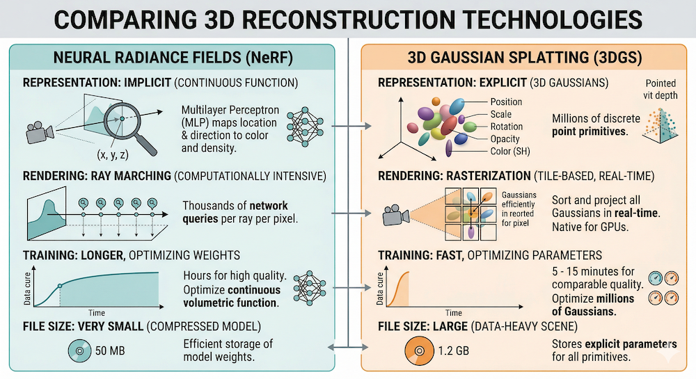
| Aspect | NeRF | 3DGS |
|---|---|---|
| Representation | Implicit (neural network) | Explicit (set of primitives) |
| Query model | Per-ray function evaluation | Rasterization (geometry pipeline) |
| Speed | 1–5 FPS | 100–300 FPS |
| Editability | Hard (weights are opaque) | Easy (splats are objects) |
| Export | Network weights | Gaussian splat file |
| GPU fit | Small models (<100 MB) | Millions of splats (100s MB–GBs) |
The speed gain comes from exploiting hardware. NeRF fights the GPU's architecture; 3DGS aligns with it.
The Rendering Pipeline: How Pixels Are Made
Rendering a single frame of a 3DGS scene is a tightly orchestrated dance on the GPU. Here's the step-by-step flow:
1. Projection: 3D Gaussian → 2D Gaussian
Each 3D Gaussian lives in world space. To render from a camera, we need its 2D projection on the image plane.
The projection involves the Jacobian of the perspective transformation applied to the 3D covariance. In mathematical notation:
where is the Jacobian of the perspective projection. Intuitively: a 3D ellipsoid, when projected through a camera lens, becomes a 2D ellipse on the image plane. Its shape and size depend on the viewing angle, distance, and the 3D ellipsoid's orientation.
This projection is differentiable—critical for optimization later.
2. Rasterize: Which Gaussians Contribute to Which Pixels?
The 2D Gaussian footprint is rasterized. For each pixel, we determine which 2D Gaussians overlap it. This is often done via tile-based rasterization: divide the image into 16×16 tiles, assign Gaussians to tiles, and process each tile independently on GPU.
3. Depth Sorting
Gaussians are sorted by their center's depth (distance from camera). Typically front-to-back, so we render near objects first, then far objects on top.
4. Alpha Compositing
For each pixel, we blend the overlapping Gaussians in order. The formula is:
where:
- is the color of Gaussian (evaluated based on viewing direction and SH)
- is the opacity of Gaussian at the pixel
- is the transmittance: how much light from this Gaussian reaches the camera
Transmittance is computed as:
where is the value of the 2D Gaussian evaluated at pixel . Intuitively: is the fraction of light that makes it through all Gaussians in front of .
5. Why It's Differentiable
Every step—projection, Gaussian evaluation, multiplication, summation—involves smooth, differentiable operations. Gradients flow backward seamlessly. This is why 3DGS can be optimized via backpropagation.
Training: From Photos to Splats
How do you actually build a 3DGS scene? You start with images and end with Gaussians.
Data Requirements
- A collection of photographs of the same scene from different viewpoints (typically 20–100+ images)
- Camera poses (position + orientation of each camera). These come from Structure-from-Motion (SfM) tools like COLMAP
Initialization
From the SfM point cloud (a sparse set of 3D points reconstructed from image pairs), initialize Gaussians:
- Position: place a Gaussian at each 3D point
- Scale, rotation, opacity, color: initialize to reasonable defaults (e.g., isotropic scale, random orientation, middle opacity)
You may start with 10k–50k Gaussians.
Optimization Loop
For each training iteration:
- Render: For each training image, render the scene from that camera pose using the current Gaussians.
- Compute loss: Compare rendered output to ground-truth image (the original photograph from that camera pose—you already have it, since it's the training data you started with). The loss is , which combines two complementary terms. is the mean absolute pixel error: for every pixel, take , then average across the image. It penalizes raw color differences and drives the Gaussians toward the correct brightness and hue. (Structural Similarity Index) is a perceptual loss that compares local patches of the rendered and ground-truth images in terms of luminance, contrast, and structure rather than raw pixel values. It catches the kind of blurriness or texture loss that alone might miss. Together, the two losses ensure the rendered image is both pixel-accurate and perceptually sharp.
- Backprop: Compute gradients of loss w.r.t. Gaussian parameters.
- Update: Step the Gaussian parameters (position, scale, rotation, opacity, SH) using an optimizer (typically Adam).
Adaptive Density Control
The magic ingredient: periodically (every N iterations), examine which Gaussians are "poorly optimized" and adjust:
- Splitting: If a Gaussian covers a large pixel footprint but has high gradient magnitude (the optimizer wants to push it hard), split it into smaller Gaussians.
- Pruning: If a Gaussian has very low opacity (nearly invisible), remove it.
- Cloning: In regions with high gradients but low Gaussian density, clone existing Gaussians.
This process grows the scene from sparse initialization to millions of Gaussians, concentrating them where needed to fit the images.
Training Time
A typical scene: 10–30 minutes on a single high-end GPU (e.g., NVIDIA A100). The bottleneck is the loss computation and backpropagation, not the number of Gaussians (once sorted and rasterized, 100k or 1M Gaussians render in similar time on modern hardware).
Why Marble Uses 3DGS
World Labs' Marble is the flagship application of 3D Gaussian Splatting technology. Here's why:
1. Explicit Representation = Editable Worlds
Unlike NeRF's implicit neural weights, Gaussian splats are objects. Marble's Chisel editor can:
- Select and move individual splats
- Delete regions
- Paint new colors
- Clone and paste
You can't do this with a neural network. Explicit geometry is editable geometry.
2. Real-Time Rendering = Interactivity
Users explore scenes at 60+ FPS. They rotate, pan, zoom without waiting. This is only possible with rasterization-based rendering. NeRF couldn't compete on responsiveness.
3. Differentiable = Generative Target
Marble is rumored to use neural models to predict Gaussian splats from images. Why? Because 3DGS is differentiable top-to-bottom:
You can train a neural network to predict Gaussians by optimizing rendered output against ground truth. NeRF can do this, but optimizing NeRF is slower (more queries per ray). Optimizing Gaussians is orders of magnitude faster. This is why the field moved.
4. Standardized Export
Scenes export as .ply files with Gaussian parameters. This is a portable, hardware-agnostic representation. Load in any renderer, edit, re-export.
Connection to W14 Theme
This week's trend tutorial dives into image-to-3D generative models that predict Gaussians. This tutorial provides the foundation: what Gaussians are, how they render, why they're the right primitive for generative 3D.
Limitations and Active Research
3DGS is not a panacea. Several frontier challenges remain:
Memory Footprint
Millions of Gaussians consume GBs of VRAM. For Marble-scale scenes (complex, photorealistic environments), memory can become a bottleneck. Compression and level-of-detail schemes are active areas of research.
Thin Structures and Fine Detail
Gaussians are blobs. They excel at soft, diffuse geometry (foliage, fabric, fur). But sharp edges, thin wires, and fine line structures are hard to represent without many Gaussians or post-processing tricks.
Dynamic Scenes
Standard 3DGS is static. Extensions like 4D-GS (for video) and Deformable 3DGS (for non-rigid motion) exist, but they add complexity and slow rendering. Capturing and rendering dynamic scenes remains more difficult than static ones. That said, the gap is closing fast: Gracia recently demonstrated 4D Gaussian splats running in real time inside the open-source PlayCanvas engine, complete with relighting and shadow casting—a sign that 4D splatting is approaching web-deployment maturity.
Lighting and Relighting
Spherical harmonics bake view-dependent appearance into the Gaussians. But they don't separate illumination from material. You can't easily relight a scene (e.g., move the sun). NeRF extensions (like Nerfacto with learnable lighting) handle this better. Recent work combines 3DGS with explicit lighting models, but it's nascent—though the Gracia + PlayCanvas demo mentioned above shows real-time relighting of Gaussian splats is now achievable in production engines.
Generalization Across Scenes
NeRF networks, when trained on diverse data, sometimes generalize to novel scenes. 3DGS splats are scene-specific; there's no implicit priors beyond the regularization in training. Generalizable 3DGS is an open problem.
Putting It Together
3D Gaussian Splatting solved the speed problem that NeRF left open. By trading implicit neural queries for explicit rasterization, the field unlocked real-time rendering, editability, and a generative-friendly output representation.
The geometry is elegant: a Gaussian is defined by five learned components (position, scale, rotation, opacity, color), each interpretable and differentiable. Rendering is a textbook rasterization pipeline, accelerated by GPUs designed for exactly this workload. Training is optimization: initialize from sparse points, render, compare to ground truth, backprop, update Gaussians, grow density where needed.
Marble exemplifies this: worlds generated by neural models, rendered in real time, edited by humans, exported as standard Gaussian splat files. This is the scaffold on which next-generation world models are built.
The techniques in the companion notebooks (NB 00: building a renderer from NumPy; NB 01: predicting Gaussians from images) show the full pipeline at a manageable scale. Start there, and the paper and production code will feel less opaque.
Further Reading
- 3D Gaussian Splatting paper: Kerbl et al. (2023)
- NeRF paper: Mildenhall et al. (2020)
- W14 Trend: Marble-Like Architectures and Generative 3D
- W13 Trend: Energy-Based World Models
- W13 Evolution: The Evolution of World Models
Stay connected:
- 📧 Subscribe to our newsletter for updates
- 📺 Watch our YouTube channel for AI news and tutorials
- 🐦 Follow us on Twitter for quick updates
- 🎥 Check us on Rumble for video content