The Image-to-3D Landscape—How One Photo Becomes a World
Map the modern image-to-3D ecosystem—from LRM-style direct regression and multi-view diffusion to latent 3D generation—and see how the frontier is now moving from static 3D to dynamic 4D worlds.
W14 Basic Tutorial 2 · Intermediate · April 2026
Research Area: 3D Generation, World Models
Companion Notebooks
| Notebook | Focus | Difficulty |
|---|---|---|
| NB 00: 3DGS From Scratch | Differentiable 3DGS renderer + optimization, pure NumPy | Intermediate |
| NB 01: Image-to-Gaussian Baseline | Minimal encoder → Gaussian decoder, toy Marble-like pipeline, NumPy CPU-only | Intermediate |
| NB 02: Novel View Synthesis | Render predicted Gaussians from new camera angles, quality-vs-angle evaluation | Intermediate |
| NB 03: Multi-View Aggregation | Fuse multiple predicted views into a single consistent 3D scene | Advanced |
The Problem: One Image, Infinite 3D Worlds
When you look at a photograph, your brain effortlessly reconstructs the 3D world behind it. You know which objects are in front, which are behind, how surfaces curve, how the scene extends beyond the frame. A neural network doesn't have this intuition.
The core challenge: A single 2D image is a projection of 3D space. Mathematically, infinite different 3D scenes could produce the exact same photograph. A cube viewed from the front looks identical to a flat square painted to look like a cube. A room with mirrors could look like a larger room. The problem is fundamentally ill-posed—there is no unique solution without additional constraints.
This is why image-to-3D is hard. The model must learn to:
- Understand geometry from context. A single image of a face teaches the model about typical head shapes, proportions, and how skin deforms.
- Hallucinate occluded regions. What is behind the person? What's under the table? The model must imagine plausible continuations.
- Maintain consistency. If the model predicts multiple views (front, side, back), they must be geometrically consistent—the edges must align, the scale must match.
Modern image-to-3D systems solve this by learning from thousands of objects, absorbing visual priors about how the world works. They trade uniqueness for plausibility: the output won't be correct, but it will be reasonable.
A Brief History: From Multi-View Stereo to Feed-Forward Models
Classical Multi-View Stereo (2000s–2010s)
Take many photographs of a scene from different angles with known camera positions. Match pixels across images to triangulate 3D points. The result: a point cloud or mesh. This is deterministic and precise—but requires many images and pre-calibrated cameras. Not generative, not single-image.
NeRF Era (2020–2022)
NeRF (Mildenhall et al., 2020) introduced neural radiance fields—a continuous function that maps 3D coordinates and viewing direction to color and density. Train one NeRF per scene by minimizing rendering loss against input images. The result: photorealistic novel views. But each scene requires hours of optimization, and there's no prior knowledge across scenes.
Diffusion-Guided Optimization (2022–2023)
DreamFusion flipped the problem: instead of training NeRFs from images, use a pretrained 2D diffusion model (like Stable Diffusion) as a critic. The key innovation was Score Distillation Sampling (SDS)—a loss function that never asks the diffusion model to see 3D at all. Instead, render the 3D representation from a random camera, add noise, and ask the 2D diffusion model "does this 2D image look like the prompt from this angle?" The gradient flows backward through the renderer, updating the 3D parameters until every projected view looks plausible. No ground-truth images needed—just language. Trade-off: slower, noisier artifacts (the now-infamous "Janus problem" of multi-faced objects), but unprecedented creative freedom.
Gaussian Splatting Speedup (2023–2024) — The Great "Explicit" Return
3DGS (Kerbl et al., 2023) replaced NeRF's implicit function with explicit 3D Gaussians—point clouds with learned covariance and color. The deeper shift was about rendering: NeRF used volume rendering, marching rays through a continuous field and querying a neural network at hundreds of points per pixel. 3DGS uses rasterization, projecting 3D ellipsoids onto the image plane and alpha-compositing them in a single pass. This is the same primitive GPUs have been optimized for since the 1990s. The result was a jump from minutes per frame (NeRF) to hundreds of frames per second (3DGS)—the speed change that made the interactive 3D worlds of 2025–2026 possible at all. DiffusionGS and similar methods then married diffusion guidance with Gaussians, keeping the creative power of SDS but with vastly faster optimization.
Feed-Forward Models (2024–2026) — The Present
Instead of optimizing per-scene, learn a single model that maps images directly to 3D in one forward pass. Two competing architectures dominate this era:
- Two-stage (multi-view diffusion → reconstructor): Models like LGM (2024) and Instant3D first use a 2D diffusion model to generate four to six consistent images of the object from canonical viewpoints, then pass those into a fast feed-forward reconstructor (Transformer or asymmetric U-Net) that converts them into Gaussians or a mesh. Higher quality, but inherits any inconsistencies the multi-view diffusion produces.
- One-stage (direct regression): Models that map the input image directly to 3D tokens or Gaussian parameters without an intermediate multi-view step. DiffusionGS is a clean example. Harder to train, but significantly faster at inference and immune to multi-view alignment errors.
The LRM Era — Scaling 3D Like Language Models
The defining trend of late 2024–2026 is the Large Reconstruction Model (LRM) architecture. Borrowing directly from LLM scaling laws, LRM (Hong et al., 2023) and its descendants are large Transformers trained on massive 3D asset datasets like Objaverse-XL (10M+ 3D objects). They treat 3D reconstruction as a sequence-to-sequence problem: image patches in, 3D tokens out. This is what enabled the leap from "generate one object" to "generate a navigable world." Systems like Marble (2025, World Labs) accept text, images, video, and panoramas—and output an interactive 3D scene in seconds. The pattern that worked for language is now working for geometry: bigger Transformers + more data + simpler losses beat clever per-scene optimization. This is where the field is now.
The Modern Pipeline: Two Architectures, One Goal
Modern feed-forward image-to-3D systems split into two families. Both share the same end goal—turn pixels into renderable Gaussians in a single forward pass—but they get there differently.
One-Stage: Direct Regression
Input Image
    ↓
[Vision Encoder: ViT / DINO patches → image tokens]
    ↓
[Large Transformer (LRM-style): cross-attend image tokens ↔ 3D tokens]
    ↓
[3D Decoder: 3D tokens → Gaussian parameters (μ, Σ, opacity, SH color)]
    ↓
[Rasterizer: project Gaussians → novel views]
    ↓
Output: Gaussian splats + renders
The image goes in, 3D tokens come out, Gaussians are decoded. No intermediate 2D images, no multi-view consistency to enforce. This is the architecture pioneered by LRM and refined by DiffusionGS. It's harder to train (the model has to learn 3D priors directly from supervised image→3D pairs) but faster at inference and immune to multi-view alignment errors.
Two-Stage: Multi-View Diffusion → Reconstructor
Input Image
    ↓
[Multi-View Diffusion Model: synthesize 4–6 canonical views]
    ↓
[Generated Views: front, back, left, right, top, bottom]
    ↓
[Feed-Forward Reconstructor (Transformer or U-Net): views → Gaussians]
    ↓
[Rasterizer: project Gaussians → novel views]
    ↓
Output: Gaussian splats + renders
Here a 2D diffusion model first hallucinates a small set of consistent views, and a fast reconstructor stitches them into 3D. This is LGM, Instant3D, and the lineage descended from Zero-1-to-3. Higher fidelity in practice (the diffusion prior is very strong), but it inherits any inconsistency the multi-view diffusion produces—and you pay the cost of two inference passes.
What's Common to Both
- Encoder. Both start with a strong vision backbone (DINO, CLIP, ViT) that turns the image into patch tokens.
- Rasterizer. Both end at the same place: a differentiable splatting renderer that projects 3D ellipsoids to 2D pixels at hundreds of FPS. This is the rasterization-vs-volume-rendering shift from the history section, and it's what makes the output interactive rather than offline.
- End-to-end training. Both pipelines are trained with rendering losses (L1 + SSIM + perceptual) against ground-truth multi-view captures, typically on Objaverse-XL-scale datasets.
The difference is whether the model regresses 3D directly or routes through a 2D diffusion intermediate.
Key Approaches: The Landscape Mapped
The field has branched into five main strategies. Each trades speed, quality, and flexibility differently. The two big winners of 2024–2026 are both feed-forward: one regresses 3D directly, the other routes through multi-view diffusion. The other three (latent 3D diffusion, video-to-3D, text-to-3D) carve out specific niches.
1. Direct Regression (One-Stage Feed-Forward)
What it is: One image in → one forward pass through a large Transformer → Gaussians out. No intermediate 2D images.
Examples: LRM (Hong et al., 2023), DiffusionGS
How it works: A vision encoder (typically a ViT) tokenizes the input image. A large Transformer cross-attends image tokens with a learned set of 3D query tokens. A lightweight decoder reads the 3D tokens out as Gaussian parameters. Train end-to-end on millions of (image, multi-view) pairs from Objaverse-XL.
Pros:
- Fastest inference. A single forward pass; no diffusion sampling loop.
- Immune to multi-view alignment errors. Nothing to align—the model never produces intermediate images.
- Scales like an LLM. More parameters + more data → monotonically better geometry. This is the LRM thesis.
- Deterministic. Same input → same output.
Cons:
- Hard to train. The model has to learn 3D priors from scratch without leaning on a pretrained 2D diffusion backbone.
- Limited geometric diversity. One viewpoint → one hypothesis. No natural way to sample alternatives.
- Hallucinates the back of objects. Looks great from the input view, often weak from 180° away.
2. Multi-View Diffusion + Reconstruction (Two-Stage Feed-Forward)
What it is: Use a 2D diffusion model to hallucinate a small set of consistent views, then run a fast reconstructor over them.
Examples: LGM (Tang et al., 2024), Instant3D (Li et al., 2023), Zero-1-to-3 (Zhou et al., 2023), SyncDreamer (Liu et al., 2023), Gen-3Diffusion (Xue et al., 2024)
How it works:
- Take one input image.
- Run a multi-view diffusion model (camera-pose-conditioned) to generate 4–6 canonical views (front, back, sides, top).
- Pass those views into a fast feed-forward reconstructor—typically an asymmetric U-Net or a Transformer—that produces Gaussians or a mesh.
Pros:
- High fidelity. Inherits the strength of pretrained 2D diffusion priors trained on billions of images.
- Better completeness. Multi-view constraints resolve occlusions.
- Easier to train. The 2D diffusion stage can be initialized from Stable Diffusion.
Cons:
- Slower. Two inference passes (diffusion + reconstructor), and diffusion sampling itself takes multiple steps.
- Inherits multi-view inconsistencies. When the diffusion model generates views that don't perfectly agree, the reconstructor has to average or hallucinate the difference. This is the source of the "blurry seam" failure mode.
- Pipeline complexity. Two models to train, two models to maintain, two models to debug.
3. Latent Diffusion in 3D Space
What it is: Skip the 2D detour entirely. Train a diffusion model directly on a learned 3D latent space.
Examples: LN3Diff (Lan et al., 2020, latent neural 3D diffusion), Complete Gaussian Splats (Liao et al., 2025)
How it works:
- Learn a VAE-like encoder/decoder for 3D scenes (Gaussian splats → latent → reconstruction).
- Train a diffusion model on the latent codes.
- Condition the 3D diffusion model on input image features and sample from the posterior.
Pros:
- Native uncertainty. Diffusion sampling gives a distribution of plausible 3D completions, not a point estimate.
- Strong geometric priors. The 3D VAE absorbs global shape statistics.
- Flexible. Can sample diverse hypotheses or take the mean.
Cons:
- Slow. Diffusion iterations in 3D latent space.
- Heavy training cost. Needs both a 3D VAE and a diffusion model trained on 3D data.
- Less mature. Smaller body of work than the two feed-forward families above.
4. Video-to-3D and the 4D Frontier
What it is: Treat a video clip as a dense multi-view capture, and either reconstruct a static 3D scene or—more ambitiously—a dynamic 4D one.
Examples: Marble (accepts video input), 4D-GS, Deformable 3DGS, World Labs RTFM
How it works: Either extract keyframes and treat them as a multi-view stack (static reconstruction), or train a model that predicts time-varying Gaussians—Gaussians whose positions, scales, and colors change frame-to-frame. The frontier is full 4D: the model predicts not just the geometry but the behavior of the scene over time.
Pros:
- Rich input signal. Video provides temporal consistency and broad coverage from one capture.
- Fast acquisition. One handheld clip beats arranging 50 photos.
- Native handle on dynamics. Objects can move, deform, or interact—not just sit still.
Cons:
- Input-quality sensitive. Needs adequate motion, lighting, and sharpness.
- Compute-heavy. 4D representations are larger and harder to optimize than static 3D.
- The hard problem of motion priors. Predicting how a scene should move requires physics or learned dynamics priors that the field is still developing.
5. Text-to-3D (Creative Applications)
What it is: No input image at all. A text prompt drives a 2D diffusion model that supervises a 3D representation.
Examples: DreamFusion (Poole et al., 2022), MVDream
How it works: Initialize a NeRF or set of Gaussians, render from random cameras, use SDS (Score Distillation Sampling) to push the renders toward what a text-conditioned diffusion model thinks they should look like. Iterate until convergence.
Pros:
- Creative freedom. Language is flexible and unconstrained—no reference image needed.
- Strong prior. The 2D diffusion model encodes visual common sense.
Cons:
- Slow. Per-scene optimization; no feed-forward shortcut.
- Janus problem. Without explicit multi-view consistency, objects often grow extra faces.
- Noisy. SDS is a noisy gradient signal; artifacts accumulate.
Landscape Comparison
| Approach | Speed | Geometry Quality | Completeness | Input | Scaling Story |
|---|---|---|---|---|---|
| 1. Direct regression (LRM-style) | Very fast | Medium–High | Medium | Image | LLM-style: scale model + data |
| 2. Multi-view diffusion + recon | Medium–Slow | High | High | Image | Inherits 2D diffusion scaling |
| 3. Latent 3D diffusion | Slow | High | High | Image | Constrained by 3D dataset size |
| 4. Video-to-3D / 4D | Fast–Medium | High | High | Video | Best with strong motion priors |
| 5. Text-to-3D (SDS) | Slow (per-scene) | Medium | Medium | Text | No feed-forward path yet |
Where Marble Fits: Inference from Public Information
Marble (World Labs, 2025) is a system that has captured significant attention. World Labs has not published a technical architecture paper, so everything below is inference from product behavior, public blog posts, and the open literature it most closely resembles.
From public information, Marble appears to:
- Accept multiple input types: text, single images, panoramas, multi-view collections, and video. This suggests a multi-encoder front end (text encoder, vision encoder, video encoder) that routes into a shared latent or token space.
- Output Gaussian splats directly. Marble renders in real time, indicating a fast explicit representation like 3DGS rather than an implicit field.
- Include a structure-first editor (Chisel). This suggests the system separates geometry reasoning from appearance—first predicting 3D layout, then adding color and material. The two-pass workflow gives artists a place to intervene before fine details are baked in.
- Render in real time with RTFM ("Real-Time Foundation Model" rendering). This implies efficient inference, almost certainly a feed-forward path rather than per-scene optimization.
- Extend to dynamic scenes. Accepting video input suggests temporal modeling, plausibly producing time-varying Gaussians (see the 4D discussion in the next section).
A reasonable hypothesis—mapping Marble onto the landscape:
Marble looks most like an LRM-class direct-regression backbone (Approach #1 above), scaled and extended along three axes:
- Multi-modal encoders feeding a shared 3D-token Transformer. Image, video, panorama, and text all get tokenized into the same sequence space, much like multi-modal LLMs do for vision and language. The Transformer body cross-attends those input tokens with a learned set of 3D query tokens that get decoded into Gaussians.
- A Chisel-style structure refinement stage. Rather than a pure single-pass model, Marble likely produces a coarse geometric layout first, exposes it for editing, then runs a second pass to add appearance. This is closer in spirit to the two-stage approach (#2)—but the "second stage" is appearance refinement rather than reconstruction from generated views.
- A 4D extension for video and dynamic worlds. RTFM and the video input strongly suggest the model produces time-varying Gaussians—the same direction 4D-GS and Deformable 3DGS are pursuing in the open literature.
Why direct regression and not multi-view diffusion? Real-time interactive output is hard to reconcile with a diffusion sampling loop in the inference path. Two-stage systems like LGM are fast in batch but still slow per request. Marble's interactivity points to a single-pass Transformer regressor—the LRM blueprint, scaled.
We emphasize: this is product analysis, not internal knowledge. Any architectural details would need to come from a published technical paper, which World Labs has not released. The point of this analysis is to show how to reason about a closed system from the open literature it most resembles—not to claim certainty about Marble's internals.
Convergence with World Models: From Image-to-3D to Image-to-4D
Image-to-3D answers one question: given a static view, what is the 3D scene?
World models (the focus of W13) answer another: given a scene, how does it change over time?
These are complementary:
- Observation (image-to-3D): 2D → 3D (static).
- Prediction (world model): 3D → 3D (dynamic).
Systems like LeWorldModel (W13's focus) predict future states in learned latent space. Marble-class systems can render those predictions as interactive 3D worlds. The trend is toward unified architectures that jointly model both observation and prediction—AMI (AI Model Integration, W13 framing) versus modular stacking (World Labs' multi-input approach). Both are valid; the field is still exploring which wins.
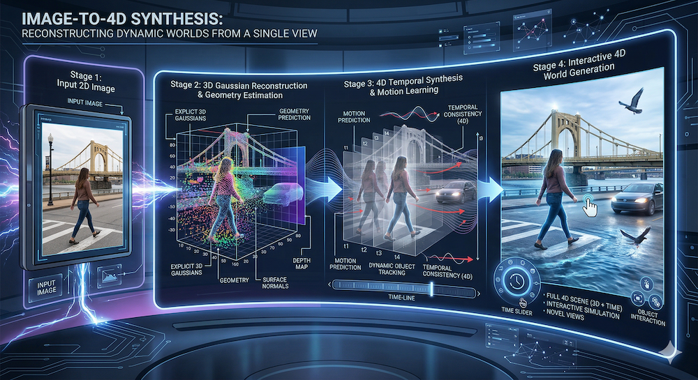
The deeper convergence is dimensional. The frontier is no longer "Image-to-3D" (static geometry); it is Image-to-4D (3D + Time). Recent work doesn't just predict the geometry of a room—it predicts how light, shadows, fluids, cloth, and rigid bodies behave inside it. 4D-GS extends Gaussian splatting to dynamic scenes. Deformable 3DGS handles non-rigid motion. World Labs' RTFM ("Real-Time Foundation Model") demonstrates real-time generation of dynamic worlds. At this point, "3D generation" has stopped being a reconstruction task and has become a simulation generation task: the model isn't producing a snapshot of a world, it's producing the rules by which that world evolves. This is where image-to-3D, world models, and physics simulation are all flowing into the same river.
What We Build: NB 01, NB 02, and NB 03 Preview
To ground this landscape, we implement a minimal image-to-3D pipeline across three notebooks—each tackling a distinct stage of the problem. All pure NumPy, CPU-only. No dependencies on external 3D libraries. The goal is to demystify the pipeline: you'll see exactly what each stage does, what gradients flow through, and how a single image becomes interactive 3D.
Notebook 01 — Image-to-Gaussian Baseline
A minimal, end-to-end image-to-3D model:
- Image encoder: A simple 2D CNN that extracts spatial features.
- Gaussian decoder: Predict 3D Gaussian parameters (centers, covariance, SH coefficients) from the latent.
- Differentiable renderer: Splatting-based rendering to a novel viewpoint.
- Loss: Render, compare to ground-truth, backprop.
This notebook demonstrates the full forward pass—from one image to a renderable 3D scene—and the engineering pitfalls of training a feed-forward image-to-3D model from scratch.
Notebook 02 — Novel View Synthesis
Once you have predicted Gaussians, how well do they actually generalize to new camera angles? NB 02 takes the output of NB 01 and stress-tests it:
- Camera orbits: Generate viewpoints around the predicted scene at varying angles and distances.
- Quality-vs-angle evaluation: Measure how rendering quality degrades as the camera rotates away from the input view.
- Smooth camera paths: Render temporally consistent video sequences and analyze flicker and pop artifacts.
The key insight: a single-image 3D model looks great from the input view—and often falls apart from the back. NB 02 makes that failure mode quantitative.
Notebook 03 — Multi-View Aggregation
NB 02 reveals the limit of single-image prediction. The natural fix: combine multiple predicted views into a single consistent 3D scene. NB 03 explores how:
- Naive fusion: Take the union of Gaussians from each predicted view and see what happens (spoiler: duplicates and inconsistencies).
- Smart fusion: Match correspondences across views, deduplicate overlapping Gaussians, and blend covariances geometrically.
- Iterative refinement: Optimize the fused scene against all views simultaneously.
This notebook bridges the gap between single-image feed-forward models and multi-view-consistent reconstruction—the same gap that systems like Gen-3Diffusion and SyncDreamer try to close at scale.
Together, the three notebooks walk the full arc: predict, evaluate, and reconcile.
Summary: The State of the Field
Image-to-3D has matured from a research curiosity (NeRF per-scene optimization) to a practical tool (feed-forward Marble, DiffusionGS, LGM, LRM-class Transformers). The arc is clear: we moved from calculating 3D (multi-view stereo) to hallucinating 3D (DreamFusion + SDS) to predicting 3D (LRM, LGM, Marble). The key insight: learn once, infer many times. Train a Transformer on millions of 3D assets, and it generalizes to novel images in milliseconds.
The remaining frontiers are:
- Geometry quality at scale. Can we maintain consistency when reconstructing complex, large-scale scenes?
- Speed vs. quality. Single-pass models are fast but approximate. Can we achieve diffusion-quality geometry without the diffusion overhead?
- User control. How do we let artists edit the output? Marble's Chisel is one answer; others are emerging.
- Temporal modeling. As systems incorporate video input and world models, predicting 3D dynamics becomes crucial.
- From 3D to 4D. The next jump is generating not just geometry but the behavior inside it—light, shadows, motion, physics. Reconstruction is becoming simulation.
The convergence of observation (image-to-3D) and prediction (world models) suggests the next era: unified generative models that understand both what exists and how it changes.
References
- 3DGS (Kerbl et al., 2023): Gaussian splatting as a fast 3D representation. https://arxiv.org/abs/2308.04079
- NeRF (Mildenhall et al., 2020): Neural radiance fields, the foundation of differentiable rendering. https://arxiv.org/abs/2003.08934
- DiffusionGS: Diffusion-guided Gaussian splatting for faster image-to-3D. https://arxiv.org/abs/2411.14384
- LGM (2024): Large Multi-View Gaussian Model for high-resolution 3D content. https://arxiv.org/abs/2402.05054
- LRM (Hong et al., 2023): Large Reconstruction Model — Transformer-based single-image to 3D reconstruction at scale. https://arxiv.org/abs/2311.04400
- Instant3D: Fast text-to-3D via two-stage multi-view diffusion + reconstruction. https://arxiv.org/abs/2311.06214
- Objaverse-XL (Deitke et al., 2023): A universe of 10M+ 3D objects, the dataset enabling LRM-scale training. https://arxiv.org/abs/2307.05663
- Gen-3Diffusion: Generation and reconstruction via multi-view diffusion. https://arxiv.org/abs/2412.06698
- Complete Gaussian Splats: Latent diffusion in 3D for incomplete-to-complete reconstruction. https://arxiv.org/abs/2508.21542
- DreamFusion (Poole et al., 2022): Text-to-3D via diffusion guidance. https://arxiv.org/abs/2209.14988
- Zero-1-to-3: Zero-shot one image to 3D object generation. https://arxiv.org/abs/2303.11328
- SyncDreamer: Multiview-consistent image generation. https://arxiv.org/abs/2309.03453
- Marble (World Labs): Real-time world generation from text, image, or video. https://www.worldlabs.ai/blog/marble-world-model
- LeWorldModel: Latent-space world models for prediction. https://arxiv.org/abs/2603.19312
Cross-References
- W14 Trend Tutorial: Marble-like architectures deep dive. https://artifocial.com/blog/marble-like-architectures-2026-apr-02
- W14 Basics (3DGS Explained): The Gaussian splatting representation. https://artifocial.com/blog/gaussian-splatting-explained-2026-apr-03
- W13 Trend Tutorial: Energy-based world models. https://artifocial.com/blog/energy-based-world-models-2026-mar-25
- W13 Landscape Basics: AMI vs. World Labs ecosystem comparison. https://artifocial.com/blog/world-labs-marble-and-landscape-2026-mar-29
Stay connected:
- 📧 Subscribe to our newsletter for updates
- 📺 Watch our YouTube channel for AI news and tutorials
- 🐦 Follow us on Twitter for quick updates
- 🎥 Check us on Rumble for video content